| Issue |
A&A
Volume 529, May 2011
|
|
|---|---|---|
| Article Number | A50 | |
| Number of page(s) | 10 | |
| Section | Planets and planetary systems | |
| DOI | https://doi.org/10.1051/0004-6361/201016144 | |
| Published online | 31 March 2011 | |
Constraining tidal dissipation in F-type main-sequence stars: the case of CoRoT-11
1
INAF-Osservatorio Astrofisico di Catania, via S. Sofia 78,
95123
Catania,
Italy
e-mail: This email address is being protected from spambots. You need JavaScript enabled to view it.
2
Research and Scientific Support Department,
European Space Agency, Keplerlaan 1, 2200AG,
Noordwijk, The
Netherlands
Received:
15
November
2010
Accepted:
18
February
2011
Abstract
Context. Tidal dissipation in late-type stars is presently poorly understood and the study of planetary systems hosting hot Jupiters can provide new observational constraints to test proposed theories.
Aims. We focus on systems with F-type main-sequence stars and find that the recently discovered system CoRoT-11 is presently the best suited for this kind of investigation.
Methods. A classic constant tidal lag model is applied to reproduce the
evolution of the system from a plausible nearly synchronous state on the zero-age main
sequence (ZAMS) to the present state, thus putting constraints on the average modified
tidal quality factor  of its F6V star.Initial
conditions with the stellar rotation period longer than the orbital period of the planet
can be excluded on the basis of the presently observed state in which the star spins
faster than the planet orbit.
of its F6V star.Initial
conditions with the stellar rotation period longer than the orbital period of the planet
can be excluded on the basis of the presently observed state in which the star spins
faster than the planet orbit.
Results. It is found that  , if the system started
its evolution on the ZAMS close to synchronization, with an uncertainty related to the
constant tidal lag hypothesis and the estimated stellar magnetic braking within a factor
of ≈5–6.For a non-synchronous initial state of the system,
, if the system started
its evolution on the ZAMS close to synchronization, with an uncertainty related to the
constant tidal lag hypothesis and the estimated stellar magnetic braking within a factor
of ≈5–6.For a non-synchronous initial state of the system,
 implies an age younger
than ~1 Gyr, while
implies an age younger
than ~1 Gyr, while  may be tested by
comparing the theoretically derived initial orbital and stellar rotation periods with
those of a sample of observed systems. Moreover, we discuss how the present value of
may be tested by
comparing the theoretically derived initial orbital and stellar rotation periods with
those of a sample of observed systems. Moreover, we discuss how the present value of
 can be
measured by a timing of the mid-epoch and duration of the transits as well as of the
planetary eclipses to be observed in the infrared with an accuracy of ~0.5–1 s
over a time baseline of ~25 yr.
can be
measured by a timing of the mid-epoch and duration of the transits as well as of the
planetary eclipses to be observed in the infrared with an accuracy of ~0.5–1 s
over a time baseline of ~25 yr.
Conclusions. CoRoT-11 is a highly interesting system that potentially
allows us a direct measure of the tidal dissipation in an F-type star as well as the
detection of the precession of the orbital plane of the planet that provides us with an
accurate upper limit for the obliquity of the stellar equator. If the planetary orbit has
a significant eccentricity ( ), it
will be possible to also detect the precession of the line of the apsides and derive
information on the Love number of the planet and its tidal quality factor.
), it
will be possible to also detect the precession of the line of the apsides and derive
information on the Love number of the planet and its tidal quality factor.
Key words: planetary systems / planet-star interactions / binaries: close / stars: late-type / stars: rotation
© ESO, 2011
1. Introduction
1.1. Tidal dissipation theories
Tidal dissipation in close binary systems with late-type components is generally constrained by the ranges of orbital periods that correspond to circular orbits as observed in clusters of different ages. Ogilvie & Lin (2007) review recent observations and conclude that the equilibrium tide theory is insufficient to explain binary circularization by at least two orders of magnitude. Therefore, in addition to the dissipation of the kinetic energy of the flow associated with the tidal bulge, which is considered in the equilibrium tide theory (e.g., Zahn 1977, 1989), other effects must be included. The dynamical tide theory treats the dissipation of waves excited by the oscillating tidal potential in the stellar interior whose kinetic energy is ultimately extracted from the orbital motion. For simplicity, we shall assume that stars are rotating rigidly.
We consider a reference frame rotating with the stellar angular velocity
Ω = 2π/Prot, where
Prot is the stellar rotation period. In that frame, the
tidal potential experienced by the star can be written as a sum of rigidly rotating
components proportional to the spherical harmonics
Ylm(θ,φ), viz.,
![Mathematical equation: \hbox{${\rm Re}\, [\Psi_{l m} r^{l} Y_{m}^{l} (\theta, \phi) \exp(-{\rm i} \hat{\omega}_{lm} t) ]$}](/articles/aa/full_html/2011/05/aa16144-10/aa16144-10-eq13.png) , where (r,θ,φ)
are spherical polar coordinates with the origin in the centre of the star,
, where (r,θ,φ)
are spherical polar coordinates with the origin in the centre of the star,
 is the tidal frequency in that frame, Ψlm the amplitude of the
component of degree l and azimuthal order m, and
t the time. The tidal frequency is given by
is the tidal frequency in that frame, Ψlm the amplitude of the
component of degree l and azimuthal order m, and
t the time. The tidal frequency is given by
 ,
where n = 2π/Porb is the
mean motion of the binary, Porb being its orbital period.
Waves are expected to be excited with the different frequencies
that correspond to the various components of the tidal potential and their amplitudes will
depend on that of the exciting component and on the response of the stellar interior. For
a nearly circular orbit, the l = m = 2 component is the
dominant one and is responsible for the synchronization of the stellar rotation with the
orbital motion (e.g., Ogilvie & Lin 2004).
,
where n = 2π/Porb is the
mean motion of the binary, Porb being its orbital period.
Waves are expected to be excited with the different frequencies
that correspond to the various components of the tidal potential and their amplitudes will
depend on that of the exciting component and on the response of the stellar interior. For
a nearly circular orbit, the l = m = 2 component is the
dominant one and is responsible for the synchronization of the stellar rotation with the
orbital motion (e.g., Ogilvie & Lin 2004).
Parameters of the transiting planetary systems having stars with Teff ≥ 6250 K.
The efficiency of tidal dissipation is usually parameterized by a dimensionless quality
factor Q proportional to the ratio of the total kinetic energy of the
tidal distortion to the energy dissipated in one tidal period
 (e.g., Zahn 2008). In the theory,
Q always appears in the combination
Q′ ≡ (3/2)(Q/k2),
where k2 is the Love number of the star that measures its
density stratification1. Therefore, the lower the
value of Q′, the stronger the tidal dissipation. In general,
Q′ depends on l, m, and the tidal
frequency
(e.g., Zahn 2008). In the theory,
Q always appears in the combination
Q′ ≡ (3/2)(Q/k2),
where k2 is the Love number of the star that measures its
density stratification1. Therefore, the lower the
value of Q′, the stronger the tidal dissipation. In general,
Q′ depends on l, m, and the tidal
frequency  ,
thus a rigorous treatment of the tidal dissipation should consider the sum of the effects
associated with the different tidal components each having its specific
Q′. In practice, we adopt a single value of Q′ that
represents an average of the contributions of the different components. Moreover, we also
average on the tidal frequency, which means averaging along the evolution of a given
system, because the tidal frequency decreases with time and goes to zero when tidal
dissipation has circularized and synchronized the binary.
,
thus a rigorous treatment of the tidal dissipation should consider the sum of the effects
associated with the different tidal components each having its specific
Q′. In practice, we adopt a single value of Q′ that
represents an average of the contributions of the different components. Moreover, we also
average on the tidal frequency, which means averaging along the evolution of a given
system, because the tidal frequency decreases with time and goes to zero when tidal
dissipation has circularized and synchronized the binary.
The observations reviewed by Ogilvie & Lin
(2007) indicate that an average Q′ ranging between
5 × 10⁵ and 2 × 10⁶ is adequate to account for the circularization
of late-type main-sequence binaries. These low values require an efficient tidal
dissipation mechanism that Ogilvie & Lin
(2007), moving along the lines of previous work, propose to be the damping of
inertial waves in the stellar interior. These waves have the Coriolis force as their
restoring force and are excited provided that the tidal frequency
satisfies the relationship  (1)The corresponding
Q′ has a remarkable dependence on the tidal and stellar rotation
frequencies owing to the complex details of wave excitation and dissipation that are still
poorly understood (cf. also Goodman & Lackner
2009). The main point, which can be regarded as firmly established, is that
Q′ decreases by 2−4 orders of magnitude when
(1)The corresponding
Q′ has a remarkable dependence on the tidal and stellar rotation
frequencies owing to the complex details of wave excitation and dissipation that are still
poorly understood (cf. also Goodman & Lackner
2009). The main point, which can be regarded as firmly established, is that
Q′ decreases by 2−4 orders of magnitude when
 with respect to the case when
  ,
because the excitation of inertial waves is forbidden in the latter case and only the
damping of the equilibrium tide contributes to the dissipation.
,
because the excitation of inertial waves is forbidden in the latter case and only the
damping of the equilibrium tide contributes to the dissipation.
In view of the present uncertainties in the dynamical tide theory, a precise determination of the tidal dissipation in binary systems with well known parameters is highly desirable. The case of F-type main-sequence stars is particularly challenging from a theoretical viewpoint because their internal structure consists of a thin outer convective zone and a radiative interior hosting a small convective core at the centre of the star. Since the propagation and dissipation of inertial waves are remarkably different in the convective and radiative zones, the study of F-type stars provides a critical test for the theory. Because the mass of the outer convection zone decreases rapidly with increasing stellar mass between 1.2 and 1.5 M⊙, the value of Q′ is expected to increase by 3−4 orders of magnitude within this mass range (Barker & Ogilvie 2009).
1.2. Testing tidal theory with planetary systems
A new opportunity to test the tidal theory comes from the star-planet systems, in particular those containing hot Jupiters. Systems with transiting planets have the best determined stellar and planetary parameters and are particularly suited to study tidal dissipation(see, e.g., Carone & Pätzold 2007). F-type host stars having a mass M ≥ 1.2−1.5 M⊙ evolve quite rapidly during their main-sequence lifetime, thus significantly improving their age estimate from model isochrone fitting in comparison with lower mass stars. A good age estimate is important to constrain the average value of Q′ by modelling the tidal evolution of a particular system (cf. Sect. 3.3). In Table 1 we list the presently known transiting systems with a star having an effective temperature Teff ≥ 6250 K, which corresponds to a spectral type earlier or equal to F8V.
The columns from left to right list the name of the system, the effective temperature
Teff, the mass M and the radius
R of the star, its rotation period Prot, as
derived from the observed spectroscopic rotation broadening
vsini and the estimated stellar radius assuming an
equator-on view of the star, the orbital period Porb, the mass
Mp and radius Rp of the planet,
the timescale for the synchronization of the stellar rotation
τsyn, and the references. To compute the synchronization
time, we assume that the entire star is synchronized as is customary in tidal theory and
is suggested by the tidal evolution of close binaries observed in stellar clusters of
different ages. The synchronization timescale is then a measure of the strength of the
tidal dissipation in the star and is computed according to the formula 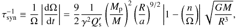 (2)where
γR ≃ 0.22 R is the gyration radius of the star
(Siess et al. 2000),
its modified
tidal quality factor, here assumed to be
(2)where
γR ≃ 0.22 R is the gyration radius of the star
(Siess et al. 2000),
its modified
tidal quality factor, here assumed to be  , a
the semimajor axis of the orbit, and G the gravitation constant (see
Mardling & Lin 2002). Equation (2) is valid for circular orbits and when the
spin axis is aligned with the orbital angular momentum. In this regard, the values given
here must be considered as estimates and for illustration purpose only, because high
eccentricity and/or obliquity have been measured for some of these systems.
, a
the semimajor axis of the orbit, and G the gravitation constant (see
Mardling & Lin 2002). Equation (2) is valid for circular orbits and when the
spin axis is aligned with the orbital angular momentum. In this regard, the values given
here must be considered as estimates and for illustration purpose only, because high
eccentricity and/or obliquity have been measured for some of these systems.
According to the dynamical tide theory by Ogilvie
& Lin (2007), the stars experiencing the strongest tidal interaction are
those with
n/Ω = Prot/Porb ≤ 2
because they have
when the l = m = 2 component of the tidal potential is
considered (Barker & Ogilvie 2009). For
these stars, the orbital decay (or expansion) owing to the tidal interaction can be
observed in principle. Among those systems, the best candidate is CoRoT-11 (Gandolfi et al. 2010) because it has a tidal
synchronization timescale in between those derived for systems like HD 197286/WASP-7 or
HAT-P-09, i.e., much longer than the main-sequence lifetime of the system, and those of,
e.g., OGLE-TR-9 or WASP-3 that are shorter than the expected ages of the systems, which
implies that the synchronous final state has possibly already been reached. Other systems,
e.g., HD15082/WASP-33, have a star so massive that a
 too large to be
measurable is expected, or show a remarkable misalignment between the stellar spin and the
orbital angular momentum that makes the derivation of the rotation period from the
vsini quite uncertain, as in the case of XO-4.
too large to be
measurable is expected, or show a remarkable misalignment between the stellar spin and the
orbital angular momentum that makes the derivation of the rotation period from the
vsini quite uncertain, as in the case of XO-4.
In view of the peculiar characteristics ofthe CoRoT-11 system, we shall consider it for a
detailed study of the tidal evolution. We shall derive constraints on the average
value of its F6V
star by considering a possible initial state for the system when its star settled on the
ZAMS (see Sect. 2.4). Moreover, we shall demonstrate
how the present value of can be
directly measured with suitable transit observations extended on a time interval of a few
decades.
2. Method: tidal evolution model and initial conditions
2.1. The constant quality-factor approximation
We adopt the classic equilibrium tidal model after Hut
(1981), in the formulation given by Leconte
et al. (2010). It assumes that the energy of the tidal perturbation raised by the
tidal potential is dissipated by viscous effects producing a constant
time lag Δt between the maximum of the tidal potential and the
tidal bulge. When Q ≫ 1,  ,
where
,
where  is the lag angle between the maximum of the deforming potential and the tidal bulge. Since
Δt is assumed to be constant during the tidal evolution,
Q and Q′ vary as
is the lag angle between the maximum of the deforming potential and the tidal bulge. Since
Δt is assumed to be constant during the tidal evolution,
Q and Q′ vary as
 .
To model the evolution of a system by assuming a constant (or, better, an average)
Q′, we need to make an approximation. Following Leconte et al. (2010), we assume for the star and the planet
.
To model the evolution of a system by assuming a constant (or, better, an average)
Q′, we need to make an approximation. Following Leconte et al. (2010), we assume for the star and the planet
 and
and
 , where the indexes s and p
refer to the star and the planet, respectively, and nobs is
the present mean orbital motion of the system corresponding to the orbital period
Porb = 2.99433 days. As we shall see (cf. Sect. 3), the mean motion n varies by a factor
of ≈4−5 during the evolution of the system, but we shall neglect this change because
we are interested in deriving the order of magnitude of the average
along the
evolution.
, where the indexes s and p
refer to the star and the planet, respectively, and nobs is
the present mean orbital motion of the system corresponding to the orbital period
Porb = 2.99433 days. As we shall see (cf. Sect. 3), the mean motion n varies by a factor
of ≈4−5 during the evolution of the system, but we shall neglect this change because
we are interested in deriving the order of magnitude of the average
along the
evolution.
The theory of dynamical tides predicts that the dissipation is a complex function of the
tidal frequency, the properties of the interior of the body, and, possibly, the strength
of the tidal potential because of non-linear effects. All these dependencies are lumped
together into the coefficients and
 and in principle
could be included in an equilibrium model provided that the relationship between their
variations along the evolution of the system and the time lag value were known. In view of
our ignorance of the processes contributing to the tidal dissipation in stars and planets
(cf., e.g., Ogilvie & Lin 2004; Goodman & Lackner 2009) and the presently
limited observational constraints, we shall consider constant, i.e. average, values of
and
and in principle
could be included in an equilibrium model provided that the relationship between their
variations along the evolution of the system and the time lag value were known. In view of
our ignorance of the processes contributing to the tidal dissipation in stars and planets
(cf., e.g., Ogilvie & Lin 2004; Goodman & Lackner 2009) and the presently
limited observational constraints, we shall consider constant, i.e. average, values of
and
 all along the
evolution and integrate the equations in Sect. 2.2 of Leconte et al. (2010) accordingly.
all along the
evolution and integrate the equations in Sect. 2.2 of Leconte et al. (2010) accordingly.
2.2. Range ofconsidered
The dynamical tide theory of Barker & Ogilvie
(2009) gives the dependence of on the tidal
and the rotation frequencies of the star when the dissipation of inertial waves is
regarded as the main source of energy dissipation – see their Fig. 8, and consider that
 for a fixed ratio
  (cf. Sect. 3.6 of Ogilvie & Lin 2007). In
view of the simplified treatment of the interaction of these waves with turbulent
convection and radiative-convective boundaries, their results can be regarded only as an
approximation of the complex dependence of on the
relevant parameters. For a star of 1.2 M⊙ and
Prot ~ 1.5 days, the average
for
can be roughly estimated to be 5 × 10⁷ with an uncertainty of at least one
order of magnitude and some preference for the lower bound because of the approximate
treatment of the above mentioned processes. Outside such a frequency range,
(cf. Sect. 3.6 of Ogilvie & Lin 2007). In
view of the simplified treatment of the interaction of these waves with turbulent
convection and radiative-convective boundaries, their results can be regarded only as an
approximation of the complex dependence of on the
relevant parameters. For a star of 1.2 M⊙ and
Prot ~ 1.5 days, the average
for
can be roughly estimated to be 5 × 10⁷ with an uncertainty of at least one
order of magnitude and some preference for the lower bound because of the approximate
treatment of the above mentioned processes. Outside such a frequency range,
 , i.e., the tidal
dissipation is reduced by at least three orders of magnitudes.
, i.e., the tidal
dissipation is reduced by at least three orders of magnitudes.
2.3. Range ofconsidered
An estimate of the tidal quality factor of the hot Jupiters may be based on astrometric
observations of the Jupiter-Io system that give  for Jupiter (see Lainey et al. 2009). Nevertheless, the quality factor
of hot Jupiters can be different from that of Jupiter owing to their different internal
structure. Assuming the observed eccentrity of the orbits of several hot Jupiters to be of
primordial origin, Matsumura et al. (2008) infer
for Jupiter (see Lainey et al. 2009). Nevertheless, the quality factor
of hot Jupiters can be different from that of Jupiter owing to their different internal
structure. Assuming the observed eccentrity of the orbits of several hot Jupiters to be of
primordial origin, Matsumura et al. (2008) infer
 , with most of
the planets having
, with most of
the planets having  . Therefore, we
shall consider
. Therefore, we
shall consider  when integrating
the equation of tidal evolution of our system. The timescale to achieve the
pseudosynchronization of the planetary rotation for CoRoT-11 and of the other systems
containing hot Jupiters is of the order of 105 yr when
when integrating
the equation of tidal evolution of our system. The timescale to achieve the
pseudosynchronization of the planetary rotation for CoRoT-11 and of the other systems
containing hot Jupiters is of the order of 105 yr when
 (cf. Sect. 2.2 of
Leconte et al. 2010). Even if
(cf. Sect. 2.2 of
Leconte et al. 2010). Even if
 this timescale is
shorter than 3 × 10⁷ yr, i.e., much shorter than the typical timescales for the
tidal evolution of the orbital parameters and the stellar spin. Therefore, we shall
consider the planet to be always in a state of pseudosynchronization, which simplifies the
integration of the tidal equations.
this timescale is
shorter than 3 × 10⁷ yr, i.e., much shorter than the typical timescales for the
tidal evolution of the orbital parameters and the stellar spin. Therefore, we shall
consider the planet to be always in a state of pseudosynchronization, which simplifies the
integration of the tidal equations.
2.4. Initial state of the tidal evolution of planetary systems
The observed distribution of the synchronization parameter n/Ω ≡ Prot/Porb provides us with information on the initial state of star-planet systems. We show n/Ω vs. the effective temperatureTeff of the host star for stars with Teff ≥ 6000 K in Fig. 1 where the most impressive feature is the lack of systems in the range 1 ≤ n/Ω ≤ 2, with the exception of HAT-P-09 and XO-3.
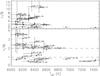 |
Fig. 1 Upper panel: the synchronization parameter n/Ω vs. the effective temperature of the star Teff in transiting planetary systems with Teff ≥ 6000 K. WASP-12 with n/Ω ≈ 33 has been omitted for the sake of clarity; lower panel: an enlargement of the lower portion of the upper panel to better show the domains close to n/Ω = 1 and n/Ω = 2, which are marked by horizontal dashed lines. The names of the systems are reported in both panels, although they are omitted for n/Ω ≤ 4.0 in the upper panel to avoid confusion. |
As conjectured by Lanza (2010), this may be
related to the processes occuring in the systems before their stars settle on the ZAMS.
After the planet forms in the circumstellar disc, it migrates inwards by transferring its
orbital angular momentum to the disc via resonant interactions (e.g., Lin et al. 1996). The migration ends where the orbital
period of the planet is half the orbital period of the particles at the inner edge of the
disc where it is truncated by the magnetic field of the protostar. Since the protostellar
magnetic field is also responsible for the locking of the stellar rotation to the inner
edge of the disc, the value of the synchronization ratio at this stage is
n/Ω ≡ Prot/Porb ≃ 2.
After a few million years, the disc disappears and the subsequent evolution depends on the
interplay between tidal and magnetic interactions coupling the star and the planet. As the
star contracts towards the ZAMS, it accelerates its rotation leading to a decrease of
n/Ω (cf. Fig. 8 of Lanza
2010). The loss of angular momentum through the stellar magnetized wind, however,
counteracts such an acceleration. If the lifetime of the disc is
 Myr,
the contraction prevails and the system enters into the domain
n/Ω < 2 characterized by a strong tidal interaction due to the
dissipation of inertial waves in the extended convective envelope of the pre-main-sequence
star (Ogilvie & Lin 2007). Angular momentum
is transferred from the orbit to the spin of the star, leading to the infall of the planet
towards the star (Hut 1980). Considering a star
similar to the Sun,
Myr,
the contraction prevails and the system enters into the domain
n/Ω < 2 characterized by a strong tidal interaction due to the
dissipation of inertial waves in the extended convective envelope of the pre-main-sequence
star (Ogilvie & Lin 2007). Angular momentum
is transferred from the orbit to the spin of the star, leading to the infall of the planet
towards the star (Hut 1980). Considering a star
similar to the Sun,  , a planet of
Mp = 1 MJ, and an orbital
period of 3 days, eq. (8) of Ogilvie & Lin
(2007) gives an infall timescale of ≈250 Myr, which may account for the lack of
systems with 1 < n/Ω < 2 given that typical stellar ages
are between ~1 and ~8 Gyr.
, a planet of
Mp = 1 MJ, and an orbital
period of 3 days, eq. (8) of Ogilvie & Lin
(2007) gives an infall timescale of ≈250 Myr, which may account for the lack of
systems with 1 < n/Ω < 2 given that typical stellar ages
are between ~1 and ~8 Gyr.
On the other hand, if the magnetic braking prevails, the system may be driven into the
domain where n/Ω > 2 and the tidal interaction becomes so weak
( ) that the planet will
spiral towards the star on a timescale much longer than the main-sequence lifetime of the
star (Ogilvie & Lin 2007), thus populating
the region of the diagram where n/Ω > 2.Only when the planet is
more massive than ~5−10 MJ and the star is
late F or cooler, the tidal interaction may lead to the infall of the planet during the
main-sequence lifetime of the star (cf., e.g., Bouchy
et al. 2011).
) that the planet will
spiral towards the star on a timescale much longer than the main-sequence lifetime of the
star (Ogilvie & Lin 2007), thus populating
the region of the diagram where n/Ω > 2.Only when the planet is
more massive than ~5−10 MJ and the star is
late F or cooler, the tidal interaction may lead to the infall of the planet during the
main-sequence lifetime of the star (cf., e.g., Bouchy
et al. 2011).
Another possible scenario occurs when the magnetic field of the pre-main-sequence star is so strong (≈3−5 kG) as to effectively couple the orbital motion of the planet to the rotation of the star after the disc has disappeared (Lovelace et al. 2008; Vidotto et al. 2010). In this case, a synchronous state is attained on a timescale of ≈2−3 Myr and maintained until the field strength decreases rapidly as the star gets close to the ZAMS. If the magnetic braking prevails over the final stellar contraction, the system would reach the ZAMS with 1 < n/Ω < 2 and the planet will eventually fall into the star owing to the strong tidal interaction. On the contrary, if the stellar contraction prevails, the star will spin up, reach n/Ω < 1 on the ZAMS, and the tides will push the planet away from the star. This may explain why several systems populate the domain n/Ω < 1 in the diagram. The present value of n/Ω is lower than the initial value on the ZAMS because the tidal interaction transfers angular momentum from the stellar spin to the planetary orbit, leading to an increase of the semimajor axis. Thus we shall base our calculations on the hypothesis that the systems observed today with n/Ω ≤ 1, as CoRoT-11, have reached the ZAMS in a state close to synchronization.
Finally, a few remarks concerning the two systems that have 1 < n/Ω < 2. The peculiar state of the HAT-P-9 system having n/Ω ≃ 1.4 may be explained by the weakness of the tidal interaction owing to the relatively small planetary mass (~0.7 MJ), and/or the young age of the system. For XO-3, the system has significant measured eccentricity and projected obliquity (e = 0.288 and λ = 37.3 ± 3.7° respectively), so it is possible that the rotation period of the star is ill estimated or that the system has undergone a different evolution.
3. Application to CoRoT-11
3.1. System parameters
Gandolfi et al. (2010) present the observations leading to the discovery of CoRoT-11 and derive the parameters of the system that are reported in their Table 4 together with their uncertainties. The stellar rotation period can be inferred only from the observed vsini and the estimated radius of the star because no evidence of rotational modulation of the optical flux has been found in the CoRoT photometry. Indeed, a modulation with a period of ≈8 days appears in the photometric time series, but it is incompatible with the maximum rotation period of 1.73 ± 0.25 days as derived from the vsini = 40.0 ± 5 km s-1 and the star radius R = 1.37 ± 0.03 R⊙. It is likely to arise from a nearby contaminant star about 2 arcsec from CoRoT-11 that falls inside the CoRoT photometric mask.
The eccentricity of the planetary orbit is ill-constrained by the radial velocity curve because of the uncertainty of the radial velocity measurements for such a rapidly rotating F-type star. An upper limit of 0.2 comes from the modelling of the transit light curve that would lead to a mean stellar density that is incompatible with a F6V star for greater values. In any case, the present radial velocity and transit data are fully compatible with a circular orbit.
The angle λ between the projections of the stellar spin and the orbital
angular momentum on the plane of the sky can be measured through the Rossiter-McLaughlin
effect (e.g., Ohta et al. 2005). Owing to the
limited precision of the available measurements, Gandolfi
et al. (2010) could not measure λ, but they established that the
planet orbits in a prograde direction, i.e., in the same direction as the stellar
rotation, and that  . An aligned
system, i.e., having λ = 0°, is compatible with their observations. The
obliquity ϵ of the stellar equator with respect to the orbital plane of
the planet is given by
cosϵ = cosIpcosi + sinIpsinicosλ,
where Ip and i are the angles of inclination
of the orbital plane and the stellar equator to the plane of the sky. Since
. An aligned
system, i.e., having λ = 0°, is compatible with their observations. The
obliquity ϵ of the stellar equator with respect to the orbital plane of
the planet is given by
cosϵ = cosIpcosi + sinIpsinicosλ,
where Ip and i are the angles of inclination
of the orbital plane and the stellar equator to the plane of the sky. Since
 ,
cosϵ ≃ sinicosλ, thus the measurement
of λ provides us with a lower limit for the obliquity of the stellar
rotation axis.
,
cosϵ ≃ sinicosλ, thus the measurement
of λ provides us with a lower limit for the obliquity of the stellar
rotation axis.
3.2. Stellar magnetic braking
Late-type stars lose angular momentum through their magnetized stellar winds. For F-type
stars, Barker & Ogilvie (2009) assumed a
braking law of the form
(dΩ/dt)mb = −γwΩ3,
where γw = 1.5 × 10⁻¹⁵ yr is a factor that accounts
for the efficiency of magnetic braking. It can be integrated to give
Ω(t) = Ω0 [1 + γwΩ0(t − t0)] -0.5,
where Ω0 is the angular velocity at initial time
t0. For Ω ≪ Ω0 this yields the usual Skumanich
braking law of stellar rotation. Applying that equation to CoRoT-11a leads to an
unrealistically fast initial rotation for an age between 1 and 3 Gyr. Indeed, the above
law of angular momentum loss does not apply to fast rotators such as CoRoT-11a for which a
saturation of the angular momentum loss rate is required to explain the observed
distribution of stellar rotation periods (cf., e.g. Bouvier
et al. 1997). Therefore, we shall assume:  , where Ωsat is the
angular velocity that corresponds to the transition to the unsaturated regime. The value
of Ωsat for solar-mass stars is ≈8 Ω⊙, where Ω⊙ is
the angular velocity of the present Sun (Irwin &
Bouvier 2009). However, its value is highly uncertain in the case of mid-F stars
because they do not show a rotational modulation measurable from the ground and experience
a remarkably lower magnetic braking than G-type stars. Considering the data in Table 4 of
Wolff & Simon (1997), we estimate a
rotation period corresponding to saturation of ≈2.8 days for mid-F stars with
vsini ~ 20−25 km s-1 at the age
of the Hyades and the adopted value of γw. However, if
CoRoT-11a is older than ~2 Gyr, the value of the saturation period must be
longer by a factor of at least ≈2, otherwise the star would have been rotating faster
than the brake-up velocity on the ZAMS. This reduction of the angular momentum loss rate
in the saturated regime can be a consequence of the initially fast angular velocity that
led to a supersaturated dynamo regime for CoRoT-11a, or an effect of the close-in massive
planet that reduced the efficiency of the stellar wind to extract angular momentum from
the star (cf. Lanza 2010).
, where Ωsat is the
angular velocity that corresponds to the transition to the unsaturated regime. The value
of Ωsat for solar-mass stars is ≈8 Ω⊙, where Ω⊙ is
the angular velocity of the present Sun (Irwin &
Bouvier 2009). However, its value is highly uncertain in the case of mid-F stars
because they do not show a rotational modulation measurable from the ground and experience
a remarkably lower magnetic braking than G-type stars. Considering the data in Table 4 of
Wolff & Simon (1997), we estimate a
rotation period corresponding to saturation of ≈2.8 days for mid-F stars with
vsini ~ 20−25 km s-1 at the age
of the Hyades and the adopted value of γw. However, if
CoRoT-11a is older than ~2 Gyr, the value of the saturation period must be
longer by a factor of at least ≈2, otherwise the star would have been rotating faster
than the brake-up velocity on the ZAMS. This reduction of the angular momentum loss rate
in the saturated regime can be a consequence of the initially fast angular velocity that
led to a supersaturated dynamo regime for CoRoT-11a, or an effect of the close-in massive
planet that reduced the efficiency of the stellar wind to extract angular momentum from
the star (cf. Lanza 2010).
3.3. Backward integration from the present state to the initial condition
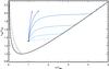 |
Fig. 2 Total angular momentum of the CoRoT-11 system in units of the critical angular
momentum as defined in Eq. (4.1) of Hut
(1980) versus the orbital mean motion in units of the present mean motion
nobs. The stellar magnetic braking law has
Psat = 6.0 days. The black solid line indicates the
total angular momentum values corresponding to tidal equilibrium. The black dotted
line represents the stability limit for the equilibrium as given by Eq. (4.2) of
Hut (1980). The solid blue lines show the
backward evolution of the system for different values of the tidal quality factor
|
We integrate the tidal evolution equations in Sect. 2.2 of Leconte et al. (2010) backwards in time starting from the present
condition, i.e., with the following parameters: stellar rotation period
Prot = 1.73 days, planet orbital period
Porb = 2.99433 days, star mass
M = 1.27 M⊙, star radius
R = 1.37 R⊙, planet mass
Mp = 2.33 MJ, planet radius
Rp = 1.43 RJ (where
MJ and RJ are the mass and
radius of Jupiter), orbital eccentricity e = 0, and stellar obliquity
ϵ = 0°. The stellar quality factor
is regarded as a
free parameter (see also Sect. 2.2).We account for
the angular momentum loss of the star due to its magnetized wind by adopting a saturated
loss rate with two possible values for
Psat = 2π/Ωsat, i.e., 6.0 or
8.0 days. Note that the results do not depend on the planet quality factor
, provided that the
orbital eccentricity is zero and the planet is assumed to be in the synchronous rotation
state.
The present state of the system and its backward evolution are represented in a tidal stability diagram similar to that of Hut (1980) in Fig. 2. The black solid line represents the value of the total angular momentum of the system when tidal equilibrium is established. For each value of the total angular momentum exceeding a minimum critical value (see Hut 1980), two equilibrium states are possible. The one on the left of the dotted line is stable, the other on the right is unstable. The filled square indicates the present state of the CoRoT-11 system with the assumption that i = 90°, i.e., the stellar rotation period is 1.73 days.
The results of the backward integrations of the tidal equations are represented by the
solid blue lines for different values of and a braking
law with Psat = 6.0 days. All the backward evolutions
asymptotically approach an initial equilibrium state where all the time derivatives of the
relevant variables vanish. Such an equilibrium is unstable, i.e., it leads to the transfer
of angular momentum from the stellar spin to the planet that is pushed outwards.
Increasing the value of the tidal
interaction weakens so that the evolution of the total angular momentum is dominated by
the magnetic braking of the star. This leads to an almost vertical evolution track in the
diagram since the star was initially rotating faster. There is no possible evolution track
that crosses the dashed line, indicating that the past system evolution has occured only
in the unstable region of the diagram, i.e., the planet has been pushed outwards starting
from its initial orbit with n/Ω < 1 during all the system
lifetime.
Given that the initial state is unstable, integrating the tidal evolution equations backwards in time is recommended to ensure the stability of the obtained solutions. The instability of the present tidal state is not a specific property of CoRoT-11, but it is generally found in hot Jupiter systems (Levrard et al. 2009), most of which evolve towards the infall of the planet into the star. Therefore, what makes CoRoT-11 peculiar is the low value of the n/Ω ratio pushing the planet outwards.
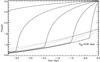 |
Fig. 3 Backward evolution of the orbital period Porb (solid
line) and the rotation period Prot (dotted line) vs.
time since the present epoch for different values of the modified tidal quality
factor |
The orbital period of the planet and the rotation period of the star are plotted vs. time
in Fig. 3 for Psat = 6.0
days. If the initial state of the system was characterized by a synchronization of the
stellar rotation with the planet orbital period, it is possible to constrain the tidal
quality factor, i.e., 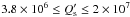 . Although we
speculated that the system may have reached the ZAMS close to synchronization in
Sect. 2.4, other evolutionary scenarios are
possible. In some of these scenarios, the planet may have started with an orbital period
longer than the stellar rotation period 3 Gyr ago, leading to the present state if
. Although we
speculated that the system may have reached the ZAMS close to synchronization in
Sect. 2.4, other evolutionary scenarios are
possible. In some of these scenarios, the planet may have started with an orbital period
longer than the stellar rotation period 3 Gyr ago, leading to the present state if
 . As an example of such
an evolution, we plot in Fig. 3 the case of
. As an example of such
an evolution, we plot in Fig. 3 the case of
 . Note that in this
case the initial state of the system has n/Ω ≃ 0.25 that is
significantly lower than the observed values of n/Ω plotted in
Fig. 1. Although the present sample of systems with
n/Ω < 1 is too small to draw conclusions on the minimum value
of n/Ω during their evolution, we hope that such a statistical
information can be used to constrain when a larger
sample is available.
. Note that in this
case the initial state of the system has n/Ω ≃ 0.25 that is
significantly lower than the observed values of n/Ω plotted in
Fig. 1. Although the present sample of systems with
n/Ω < 1 is too small to draw conclusions on the minimum value
of n/Ω during their evolution, we hope that such a statistical
information can be used to constrain when a larger
sample is available.
On the other hand,  implies a system
younger than ~1 Gyr. To illustrate this point, we plot in Fig. 3 the evolution for
implies a system
younger than ~1 Gyr. To illustrate this point, we plot in Fig. 3 the evolution for
 for which the
system reached synchronization ~0.4 Gyr ago. Although the backward evolution
can be continued to earlier times, this initial state is unstable as well as all the
allowed initial states with
Porb > Prot. For
, the tidal interaction
would be so strong and the evolution so fast that the system would reach a present value
of Porb longer than observed. Therefore, we can set a lower
limit on on the basis
of the estimated age of the system. Note that if the system were younger than
~0.7−1 Gyr, the value could
be so low that we might directly measure it after a few decades of timing observations
(see Sect. 4).
for which the
system reached synchronization ~0.4 Gyr ago. Although the backward evolution
can be continued to earlier times, this initial state is unstable as well as all the
allowed initial states with
Porb > Prot. For
, the tidal interaction
would be so strong and the evolution so fast that the system would reach a present value
of Porb longer than observed. Therefore, we can set a lower
limit on on the basis
of the estimated age of the system. Note that if the system were younger than
~0.7−1 Gyr, the value could
be so low that we might directly measure it after a few decades of timing observations
(see Sect. 4).
The evolution tracks obtained for Psat = 8.0 days and
different values of the average are plotted
in Fig. 4. They show that a decrease of the braking
rate of CoRoT-11a by ~30 percent leads to a comparable decrease in the values
of the average because a
stronger tidal interaction is needed to transfer the required amount of angular momentum
from the stellar spin to the planet when the stellar rotation was initially slower. On the
other hand, if we adopt Psat = 2.8 days, as estimated from the
data of Wolff & Simon (1997), the stellar
braking was so rapid that only for a system younger than 1 Gyr we may find an acceptable
evolution with  . For higher values of
, the
evolution takes longer, and this leads to a planet approaching the Roche lobe radius
and/or an initial stellar rotation exceeding the break-up velocity. Therefore, the
assumption that Psat is at least ~5−6 days seems
to be more likely for CoRoT-11a than Psat ~ 3−4
days. In the latter case, the system would be so young and the average
so small that
we expect to detect the tidal increase of the orbital period within a few decades (see
Sect. 4).
. For higher values of
, the
evolution takes longer, and this leads to a planet approaching the Roche lobe radius
and/or an initial stellar rotation exceeding the break-up velocity. Therefore, the
assumption that Psat is at least ~5−6 days seems
to be more likely for CoRoT-11a than Psat ~ 3−4
days. In the latter case, the system would be so young and the average
so small that
we expect to detect the tidal increase of the orbital period within a few decades (see
Sect. 4).
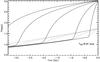 |
Fig. 4 Backward evolution of the orbital period Porb (solid
line) and the rotation period Prot (dotted line) vs.
time since the present epoch for different values of the modified tidal quality
factor |
3.3.1. Initial eccentricity of the orbit
In the scenario introduced in Sect. 2.4, the
initial eccentricity of the planetary orbit would be close to zero (Sari & Goldreich 2004), unless an encounter
with some planetary or stellar body would have excited it. Assuming that no third body
has been perturbing the system after that event, the evolution of any primordial
eccentricity is ruled by the dissipation inside both the star and the planet, the latter
being the most important for  . The timescale
for the damping of the eccentricity
. The timescale
for the damping of the eccentricity  adopting the present parameters of the system is ~120 Myr for
e = 0.2,
adopting the present parameters of the system is ~120 Myr for
e = 0.2,  , and
, and
 , and increases to
~1.1 Gyr for
, and increases to
~1.1 Gyr for  . Since the tidal
interaction was initially stronger – it scales as a-5 – the
initial τe was one order of magnitude shorter than the above
values, leading to a rapid damping of any initial eccentricity, unless
. Since the tidal
interaction was initially stronger – it scales as a-5 – the
initial τe was one order of magnitude shorter than the above
values, leading to a rapid damping of any initial eccentricity, unless
 . Moreover, for
initially high eccentricities (i.e.,
. Moreover, for
initially high eccentricities (i.e.,  )
and an initial n/Ω ≈ 1, the evolution of the system may be
significantly affected and the infall of the planet occurs as the orbital angular
velocity at the periastron exceeds the stellar angular velocity. To prevent such an
infall, we must assume that the star was initially rotating remarkably faster than
considered above. Because the rotation braking on the main sequence is expected to be
small, this is hardly compatible with the present estimated rotation period. We conclude
that the present eccentricity of CoRoT-11 is likely to be close to zero. In any case, we
describe in Sect. 4 observations that can
constrain the present value of e to allow us to distinguish among
different scenarios for the system evolution.
)
and an initial n/Ω ≈ 1, the evolution of the system may be
significantly affected and the infall of the planet occurs as the orbital angular
velocity at the periastron exceeds the stellar angular velocity. To prevent such an
infall, we must assume that the star was initially rotating remarkably faster than
considered above. Because the rotation braking on the main sequence is expected to be
small, this is hardly compatible with the present estimated rotation period. We conclude
that the present eccentricity of CoRoT-11 is likely to be close to zero. In any case, we
describe in Sect. 4 observations that can
constrain the present value of e to allow us to distinguish among
different scenarios for the system evolution.
3.3.2. Initial obliquity of the orbit
The obliquity of the CoRoT-11 system may be significantly different from zero, as
indeed found for several stars accompanied by hot Jupiters with
Teff > 6250 K (Winn
et al. 2010). For a system born close to n/Ω = 1, we need
Ωcosϵ > n to prevent the tidal infall of the
planet, and the observational result that CoRoT-11 is compatible with an aligned system
agrees with this constraint. Initial values of the obliquity
ϵ > 30° require a fast-rotating star, which is difficult to
reconcile with the presently observed vsini and
stellar radius. However, lower values of the obliquity cannot be excluded. They are
damped on a timescale that depends on the value of
, as
illustrated in Fig. 5 where the time has been
scaled inversely to the stellar tidal quality factor. These plots show that after an
initial remarkable damping of the obliquity, it asymptotically approaches a value about
half its initial value that practically corresponds to the present value. In Sect. 4 we shall discuss how this value can be constrained
with accurate timing observations of the system.
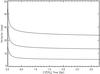 |
Fig. 5 Forward evolution of the obliquity from the ZAMS for different initial values of the angle itself. The planetary orbit is assumed circular and the initial orbital period is 0.7 days, while the initial rotation period of the star is 0.48 days for ϵ(t = 0) = 45°, 0.60 days for ϵ(t = 0) = 30°, and 0.67 days for ϵ(t = 0) = 15°, to prevent the infall of the planet. |
4. Measuring the present tidal dissipation
The main conclusion of the previous section is that the mean modified tidal quality factor
of CoRoT-11a  , provided that the
system started its evolution on the ZAMS from a nearly synchronous state. Since
is subject to
remarkable variations during the evolution of the system, this result is of limited value to
constrain dynamical tide theory, as for the mean values of
derived from
close binaries in clusters. However, a much more interesting opportunity offered by CoRoT-11
is the possibility to measure the present value of from the rate
of orbital period variation. Moreover, as we shall see, the rate of orbital period variation
also depends on the orbit parameters, and we can extract a wealth of information from
CoRoT-11 using the timing method.
, provided that the
system started its evolution on the ZAMS from a nearly synchronous state. Since
is subject to
remarkable variations during the evolution of the system, this result is of limited value to
constrain dynamical tide theory, as for the mean values of
derived from
close binaries in clusters. However, a much more interesting opportunity offered by CoRoT-11
is the possibility to measure the present value of from the rate
of orbital period variation. Moreover, as we shall see, the rate of orbital period variation
also depends on the orbit parameters, and we can extract a wealth of information from
CoRoT-11 using the timing method.
4.1. The circularized and aligned system hypothesis
If the present orbit is circular, the semimajor axis is subject to a secular increase
because the star is rotating faster than the orbital motion of the planet, so angular
momentum is transferred from the stellar spin to the orbit via the tidal interaction. When
e = 0 and the stellar obliquity is negligible
(ϵ ~ 0°), the rate of this transfer depends on the system
parameters, which are known to a good level of precision, and on
only. Therefore, we
can compute the rate of orbital period increase
dPorb/dt and use it to derive the
difference (O–C) between the observed time of mid-transit and that computed with a
constant period ephemeris after N orbital periods, viz.: 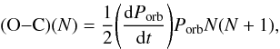 (3)where we have
assumed that the constant period of the ephemeris is the orbital period at
N = 0, i.e., at the epoch of the first transit. Using the tidal
evolution model of Leconte et al. (2010) and
assuming e = 0, ϵ = 0°, and the maximum stellar rotation
period Prot = 1.73 days, we find:
(3)where we have
assumed that the constant period of the ephemeris is the orbital period at
N = 0, i.e., at the epoch of the first transit. Using the tidal
evolution model of Leconte et al. (2010) and
assuming e = 0, ϵ = 0°, and the maximum stellar rotation
period Prot = 1.73 days, we find: 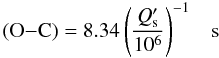 (4)after
N = 3000 orbital periods, i.e., 24.6 years.
(4)after
N = 3000 orbital periods, i.e., 24.6 years.
The epoch of mid transit can be determined with an accuracy that depends on the depth and
duration of the transit, the accuracy of the photometry, and the presence of noise
sources, e.g., related to stellar activity. In the case of CoRoT-11, because the star
shows no signs of magnetic activity, the precision of the transit timing is dominated by
the photometric accuracy. Gandolfi et al. (2010)
report in their Table 4 a precision of ~25 s for the initial epoch of their
ephemeris as obtained from a sequence of ~50 transits observed with a
photometric accuracy of ~250 parts per million (ppm) and a cadence of
~130 s. Recently, Winn et al. (2009)
using the Magellan/Baade 6.5-m telescope, observed two transits of the hot Jupiter
WASP-4b, reaching a photometric accuracy of ~500 ppm (standard deviation) in
their individual measurements obtained with a cadence of 30 s. The average standard
deviation of the epoch of mid-transit is ~5 s, which can be assumed as the
limit presently attainable with ground-based photometry. The transit of WASP-4b has a
depth of ≈0.028 mag and the star has a magnitude of V ≃ 12.5, while
that of CoRoT-11 has a depth of ≈0.011 mag and the star has V = 12.94.
Therefore, it is reasonable to assume that a timing accuracy of 0.5−1 s can be reached
with a space-borne dedicated telescope of aperture 2−3 m, since the precision is
expected to scale with the accuracy of the photometry that should reach 200−300 ppm in
~15 s integration time. This instrument would allow us to detect the expected
transit time variation (hereafter TTV) with 3σ significance after an
interval of ~25 years for  . Even if no
significant TTV is detected, a stringent lower limit can be placed on
, with the
sensitivity increasing as the square of the considered time baseline (cf. Eq. (3)).
. Even if no
significant TTV is detected, a stringent lower limit can be placed on
, with the
sensitivity increasing as the square of the considered time baseline (cf. Eq. (3)).
4.2. The eccentric system hypothesis
A significant eccentricity of the planetary orbit can affect the O–C of the TTV,
particularly when tidal dissipation in the planet is not negligible. This happens because
the angular momentum of the planetary orbit is given by
![Mathematical equation: \hbox{$L_{\rm p} = [(M_{\rm s} M_{\rm p}/(M_{\rm s} + M_{\rm p})] n a^{2} \sqrt{1- e^{2}}$}](/articles/aa/full_html/2011/05/aa16144-10/aa16144-10-eq217.png) ,
so an increase of Lp does not necessarily lead to an increase
of a when the eccentricity is damped. Assuming e = 0.2,
, and
,
so an increase of Lp does not necessarily lead to an increase
of a when the eccentricity is damped. Assuming e = 0.2,
, and
 , we find
O−C = −8.33 s after 24.6 yr, owing to the strong dissipation inside the planet that
dumps the eccentricity with a timescale of ~120 Myr. If the dissipation inside
the planet is weaker, the absolute value of the O–C decreases. For instance, if
, we find
O−C = −8.33 s after 24.6 yr, owing to the strong dissipation inside the planet that
dumps the eccentricity with a timescale of ~120 Myr. If the dissipation inside
the planet is weaker, the absolute value of the O–C decreases. For instance, if
 , we obtain
O–C = 0.49 s after 24.6 yr.
, we obtain
O–C = 0.49 s after 24.6 yr.
Furthermore, if the orbit of CoRoT-11 is indeed eccentric, the measurement of the O–C of
the primary transit are not sufficient to determine
. This happens
because in addition to the tidal evolution, also the precession of the line of the apsides
(due to the planetary and stellar tidal deformations and general relativistic effects)
produces a TTV (see Miralda-Escudé 2002; Ragozzine & Wolf 2009). For
e = 0.2, and a planet Love number k2 = 0.3,
similar to that of Saturn, we have a precession period of only ~3300 yr, which
leads to a maximum O−C = 18.1 s after N = 3000 orbital periods, i.e.,
24.6 yr. To separate the effects of the apsidal precession from those of tidal origin, we
note that the apsidal precession produces an oscillation of the O–C of the mid of the
secondary eclipse, i.e., when the planet is occulted by the star, which is always shifted
in phase by 180° with respect to that of the primary transit. In other words, the two
oscillations have always opposite signs, as is well known for the apsidal precession of
close binaries (see, e.g., Gimenez et al. 1987). On
the other hand, the O–C of tidal origin has the same sign for both the primary transit and
the secondary eclipse, so it can be separated from that arising from apsidal precession.
We conclude that a measurement of the eccentricity (or a determination of a more
stringent upper limit) is critical to derive from the
O–C observations. A direct constraint on the eccentricity can be obtained from the
observation of the time of the secondary eclipse. Gandolfi
et al. (2010) did not find evidence of a secondary eclipse in the CoRoT light
curve, which sets an upper limit of ~100 ppm to its depth in the spectral range
300−1100 nm. However, it should be possible to detect the secondary eclipse in the
infrared, thus deriving the value of ecosω, where
ω is the longitude of the periastron, from the deviation of the time of
the secondary eclipse from half the orbital period. For HD 189733 Knutson et al. (2007) found, observing in a band centred at
8 μm with IRAC onboard of Spitzer, that the secondary eclipse occurred
120 ± 24 s after the time expected for a circular orbit, leading to
ecosω = 0.001 ± 0.0002. The same method has been
applied to constrain the eccentricity of the orbit of CoRoT-2 finding
ecosω = −0.00291 ± 0.00063 (Gillon et al. 2010). Moreover, the duration of the primary transit and
the secondary eclipse can provide a measurement of
esinω, although with a precision significantly poorer
than for the secondary eclipse timing (see Sect. 2.5 of Ragozzine & Wolf 2009). In conclusion, we recommend to perform infrared
photometry of CoRoT-11 to constrain its orbital eccentricity.
The present fast rotation of CoRoT-11a can in principle excite the eccentricity of the
orbit during the phase of the evolution when
Prot/Porb < 11/18
(cf. Eq. (6) of Leconte et al. 2010). However, the
tidal dissipation inside the planet is effective at damping the eccentricity and only for
 we find an increasing
eccentricity for the present state of the system.Imposing that the eccentricity is always
damped along the past evolution of the system, we find
we find an increasing
eccentricity for the present state of the system.Imposing that the eccentricity is always
damped along the past evolution of the system, we find
 for
for
 .
.
4.3. Non-negligible obliquity hypothesis
If the present obliquity of the system is not negligible, the rate of orbital period
increase and the corresponding O–C in Eq. (4) must be multiplied by 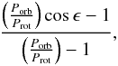 (5)because the
component of the stellar angular momentum interacting with the orbit is
Lscosϵ, where
Ls is the modulus of the angular momentum of the star (cf.
Eq. (2) of Leconte et al. 2010).
(5)because the
component of the stellar angular momentum interacting with the orbit is
Lscosϵ, where
Ls is the modulus of the angular momentum of the star (cf.
Eq. (2) of Leconte et al. 2010).
It is interesting to note that the obliquity can be constrained not only through the observation of the Rossiter-McLaughlin effect, but also by measuring the precession of the orbital plane of the planet around the total angular momentum of the system that is expected when ϵ ≠ 0°. This precession arises because the stellar gravitational quadrupole moment is non-negligible owing to its fast rotation. More precisely, adopting a stellar Love number k2s = 0.0138 after Claret (1995) and Prot = 1.73 days, we find J2 = 4.19 × 10⁻⁵. The contribution to J2 arising from the tidal deformation of the star induced by the planet is about 1100 times smaller and can be safely neglected.
Even assuming an obliquity of a few degrees, the precession period is so short as to give
measurable effects. For instance, for ϵ = 5°, the precession of the
orbital plane has a period of ~7.0 × 10⁴ years, according to Eq. (4)
of Miralda-Escudé (2002). This produces a variation
of the length of the transit chord across the disc of the star that leads to a variation
of the transit duration (transit duration variation, hereafter TDV). Applying Eq. (12) of
Miralda-Escudé (2002) and assuming that the total
angular momentum of the system is approximately perpendicular to the line of sight, we
find a maximum TDV of ~8 s in one year. Assuming a precision of
~40 s in the measurement of the duration of the transit as obtained with CoRoT
observations, this variation should be easily detected in ~5 yr and can provide
a lower limit for the stellar obliquity, which is remarkably better than what is
achievable with the Rossiter-McLaughlin effect if  .
.
5. Role of a possible third body
The use of TTV to measure the tidal dissipation inside the star (and the planet, in the case of an eccentric orbit) can be hampered by the presence of a distant third body that induces apparent O–C variations owing to the light-time effect related to the revolution of the star-planet system around the common centre of mass. In principle, any light-time effect induced by a third body is periodic while the effects of tidal dissipation are secular, i.e., they do not change sign. However, if the orbital period of the third body around the barycentre of the system is longer than, say, three times the time baseline of our observations, it may become difficult or impossible to separate the two effects.
To be specific, let us consider an O–C of 3 s observed with a time baseline of ΔT ~ 25 yr. If it is caused by a light-time effect, the corresponding radial motion of the star-planet system is Δz = c(O−C) ~ 109 m, where c is the speed of light, and the radial velocity of the barycentre of the system is Δz/ΔT ≃ 1.26 m s-1, too small to be detectable with the present radial velocity accuracy (cf. Gandolfi et al. 2010). A third body moving on a coplanar circular orbit with a period of, say, Ptb = 75 yr, would have an orbital semimajor axis of ~2.88 × 10¹² m and a minimum mass of 0.2 MJ to induce a reflex motion of the above amplitude. Its direct detection is very difficult because its apparent separation from the central star would be only 0.034 arcsec, given an estimated distance to CoRoT-11 of 560 ± 30 pc. Astrometric measurements with the GAIA or SIM satellites cannot be used to detect the reflex motion of CoRoT-11 because it would correspond to a maximum displacement of only ~2.4 μarcsec during an interval of 5 yr, which is impossible to separate from the much larger proper motion of the system.
If the orbit of the third body is inclined to the orbital plane of the star-planet system, the orbital plane of the planet will precede around the total angular momentum of the system. Assuming a third body mass of 0.2 MJ, a relative inclination of the orbits of 45°, and a semimajor axis of ~2.88 × 10¹² m, equal to ~20 AU, Eq. (8) of Miralda-Escudé (2002) gives a precession period of ~14 Gyr, i.e., too long to be observable.
Secular perturbations of the orbit of the planet by the distant third body can be neglected because they induce a variation of the O–C of the order of Porb/Ptb ~ 10-4 of the light-time effect (cf., e.g., Borkovits et al. 2003). On the other hand, a perturber on a close-in orbit, possibly in resonance with the planet, would induce O–C variations with a short periodicity and an amplitude up to a few minutes (Agol et al. 2005), which would be easily detectable.
It is interesting to note that CoRoT-11a has a low level of magnetic activity in contrast to stars with lower effective temperature. This implies that the orbital period modulation induced by magnetic activity (Lanza et al. 1998; Lanza 2006) can be excluded as a source of O–C variations in this case. This is not possible for cooler stars (Watson & Marsh 2010) which are therefore less suitable to measure the TTV induced by tidal dissipation.
6. Conclusions
Assuming an initial state of the CoRoT-11 system close to synchronization between the
stellar spin and the orbital period of the planet, we can put constraints on the average
modified tidal quality factor of its F-type star, finding
 . Rigorously speaking, we
should have expressed these constraints in terms of the average tidal time lag
Δt because our tidal equations are valid for a constant
Δt (cf. Sect. 2 and Leconte et al. 2010). However, in view of the uncertainty
on the above constraints, we prefer to give them in terms of
that varies by
a factor up to ≈4−5 during the evolution, if Δt is assumed to be
constant (cf. Sects. 2 and 3.3).
. Rigorously speaking, we
should have expressed these constraints in terms of the average tidal time lag
Δt because our tidal equations are valid for a constant
Δt (cf. Sect. 2 and Leconte et al. 2010). However, in view of the uncertainty
on the above constraints, we prefer to give them in terms of
that varies by
a factor up to ≈4−5 during the evolution, if Δt is assumed to be
constant (cf. Sects. 2 and 3.3).
An initial state close to synchronization is not the only possible one. However, the
minimum estimated age of the system of ~1 Gyr implies
 , otherwise the evolution
from any initial state with
Porb > Prot would be too
fast, leading to a present Porb longer than observed. An upper
limit on can be set when
a larger statistics of the values of the
n/Ω = Prot/Porb
ratio will be available because for
, otherwise the evolution
from any initial state with
Porb > Prot would be too
fast, leading to a present Porb longer than observed. An upper
limit on can be set when
a larger statistics of the values of the
n/Ω = Prot/Porb
ratio will be available because for  the initial value of
n/Ω is predicted to be ~0.25 that is smaller than the
presently observed minimum n/Ω ~ 0.5 (see Sect. 3.3).
the initial value of
n/Ω is predicted to be ~0.25 that is smaller than the
presently observed minimum n/Ω ~ 0.5 (see Sect. 3.3).
The above limits on are only a
factor of 2−15 smaller than the average value predicted by Barker & Ogilvie (2009), which can be considered a success of the dynamic
tide theory of Ogilvie & Lin (2007) given the
current uncertainty on the tidal dissipation processes occurring in stellar convection
zones.
We find that CoRoT-11 is one of the best candidates to look for orbital period variations
related to tidal evolution by monitoring its transits and secondary eclipses in the optical
and in the infrared passbands. In contrast to several systems hosting very hot Jupiters,
e.g., WASP-12 or WASP-18, whose orbital decay may be too slow to be measurable (Ogilvie & Lin 2007; Li et al. 2010), the parameters of CoRoT-11 appear to be ideal for a
detection by measuring the times of mid-transit and mid-eclipse with an accuracy of at least
1−5 s along a time baseline of ~25 yr. This is a consequence of the peculiar
ratio of the rotation period of the star to the orbital period of the planet that is
presently the smallest among systems having a radial velocity curve compatible with zero
eccentricity. The test is particularly sensitive to values of
between
105 and 106, leading to a fast tidal evolution of the system, as
discussed in Sect. 3.3.
The CoRoT-11 system is also particular because the precession of the orbital plane due to a
non-zero obliquity of the stellar spin can be measured through the variation of the duration
of the transit on a timescale as short as 5−10 yr by means of ground-based observations
with telescopes of the 6−8 m class. Note that even an obliquity as low as 5° can be
detected with this method. On the other hand, the eccentricity of the planetary orbit can be
well constrained by measuring the times of the secondary eclipses in the infrared and their
duration. If the system turns out to have an eccentric orbit, this puts a constraint also on
the minimum value of the planet quality factor if we assume
that the eccentricity is of primordial origin, or is a clear indication of the presence of a
perturbing body that excites it (e.g., Takeda &
Rasio 2005). The light-time effect caused by a distant third body is indeed the
only phenomenon that can seriously hamper the detection of the transit time variations
expected from the tidal orbital evolution. The detection of a distant companion may be
particularly difficult, but this limitation is present also in any other system candidate
for a direct measurement of the tidal dissipation.
Note that k2 is twice the apsidal motion constant of the star, often indicated with the same symbol, as in, e.g., Claret (1995).
Acknowledgments
The authors are grateful to the referee, Prof. J.-P. Zahn, for several valuable comments on the first version of the manuscript, and to Drs. L. Carone and S. Ferraz-Mello for interesting discussions. Active star research and exoplanetary studies at INAF-Catania Astrophysical Observatory and the Department of Physics and Astronomy of Catania University are funded by MIUR (Ministero dell’Istruzione, Università e Ricerca) and by Regione Siciliana, whose financial support is gratefully acknowledged. This research made use of the ADS-CDS databases, operated at the CDS, Strasbourg, France.
References
- Agol, E., Steffen, J., Sari, R., & Clarkson, W. 2005, MNRAS, 359, 567 [NASA ADS] [CrossRef] [Google Scholar]
- Ammler-von Eiff, M., Santos, N. C., Sousa, S. G., et al. 2009, A&A, 507, 523 [NASA ADS] [CrossRef] [EDP Sciences] [Google Scholar]
- Anderson, D. R., Hellier, C., Gillon, M., et al. 2010, ApJ, 709, 159 [NASA ADS] [CrossRef] [Google Scholar]
- Bakos, G. Á., Kovács, G., Torres, G., et al. 2007, ApJ, 670, 826 [NASA ADS] [CrossRef] [Google Scholar]
- Barker, A. J., & Ogilvie, G. I. 2009, MNRAS, 395, 2268 [NASA ADS] [CrossRef] [Google Scholar]
- Borkovits, T., Érdi, B., Forgács-Dajka, E., & Kovács, T. 2003, A&A, 398, 1091 [NASA ADS] [CrossRef] [EDP Sciences] [Google Scholar]
- Bouchy, F., Deleuil, M., Guillot, T., et al. 2011, A&A, 525, A68 [NASA ADS] [CrossRef] [EDP Sciences] [Google Scholar]
- Bouvier, J., Forestini, M., & Allain, S. 1997, A&A, 326, 1023 [NASA ADS] [Google Scholar]
- Cameron, A. C., Guenther, E., Smalley, B., et al. 2010, MNRAS, 407, 507 [NASA ADS] [CrossRef] [Google Scholar]
- Carone, L., & Pätzold, M. 2007, Planet. Space Sci., 55, 643 [NASA ADS] [CrossRef] [Google Scholar]
- Claret, A. 1995, A&AS, 109, 441 [NASA ADS] [Google Scholar]
- Cohen, O., Drake, J. J., Kashyap, V. L., Sokolov, I. V., & Gombosi, T. I. 2010, ApJ, 723, L64 [NASA ADS] [CrossRef] [Google Scholar]
- Gandolfi, D., Hébrard, G., Alonso, R., et al. 2010, A&A, 524, A55 [NASA ADS] [CrossRef] [EDP Sciences] [Google Scholar]
- Gibson, N. P., Pollacco, D., Simpson, E. K., et al. 2008, A&A, 492, 603 [NASA ADS] [CrossRef] [EDP Sciences] [Google Scholar]
- Gillon, M., Lanotte, A. A., Barman, T., et al. 2010, A&A, 511, A3 [NASA ADS] [CrossRef] [EDP Sciences] [Google Scholar]
- Gimenez, A., Kim, C.-H., & Nha, I.-S. 1987, MNRAS, 224, 543 [NASA ADS] [CrossRef] [Google Scholar]
- Goodman, J., & Lackner, C. 2009, ApJ, 696, 2054 [NASA ADS] [CrossRef] [Google Scholar]
- Hebb, L., Cameron, A. C., Loeillet, B., et al. 2009, ApJ, 693, 1920 [NASA ADS] [CrossRef] [Google Scholar]
- Hellier, C., Anderson, D., Gillon, M., et al. 2009a, ApJ, 690 , L89 [NASA ADS] [CrossRef] [Google Scholar]
- Hellier, C., Anderson, D. R., Cameron, A. C., et al. 2009b, Nature, 460, 1098 [NASA ADS] [CrossRef] [Google Scholar]
- Hut, P. 1980, A&A, 92, 167 [NASA ADS] [Google Scholar]
- Hut, P. 1981, A&A, 99, 126 [NASA ADS] [Google Scholar]
- Irwin, J., & Bouvier, J. 2009, IAU Symp., 258, 363 [NASA ADS] [Google Scholar]
- Jenkins, J. M., Borucki, W. J., Koch, D. G., et al. 2010, ApJ, 724, 1108 [NASA ADS] [CrossRef] [Google Scholar]
- Johns-Krull, C. M., McCullough, P. R., Burke, C. J., et al. 2008, ApJ, 677, 657 [NASA ADS] [CrossRef] [Google Scholar]
- Johnson, J., Winn, J., Albrecht, S., et al. 2009, PASP, 121, 1104 [NASA ADS] [CrossRef] [Google Scholar]
- Joshi, Y., Pollacco, D., Cameron, A. C., et al. 2008, MNRAS, 392 , 1532 [Google Scholar]
- Kipping, D. M., Bakos, G. Á., Hartman, J., et al. 2010, ApJ, 725, 2017 [NASA ADS] [CrossRef] [Google Scholar]
- Koch, D. G., Borucki, W. J., Rowe, J. F., et al. 2010, ApJ, 713, L131 [NASA ADS] [CrossRef] [Google Scholar]
- Knutson, H. A., Charbonneau, D., Allen, L. E., et al. 2007, Nature, 447, 183 [NASA ADS] [CrossRef] [PubMed] [Google Scholar]
- Lainey, V., Arlot, J.-E., Karatekin, Ö., & van Hoolst, T. 2009, Nature, 459, 957 [NASA ADS] [CrossRef] [PubMed] [Google Scholar]
- Lanza, A. F. 2006, MNRAS, 369, 1773 [NASA ADS] [CrossRef] [Google Scholar]
- Lanza, A. F. 2010, A&A, 512, A77 [NASA ADS] [CrossRef] [EDP Sciences] [Google Scholar]
- Lanza, A. F., Rodonò, M., & Rosner, R. 1998, MNRAS, 296, 893 [NASA ADS] [CrossRef] [Google Scholar]
- Leconte, J., Chabrier, G., Baraffe, I., & Levrard, B. 2010, A&A, 516, A64 [NASA ADS] [CrossRef] [EDP Sciences] [Google Scholar]
- Levrard, B., Winisdoerffer, C., & Chabrier, G. 2009, ApJ, 692, L9 [NASA ADS] [CrossRef] [Google Scholar]
- Li, S.-L., Miller, N., Lin, D. N. C., & Fortney, J. J. 2010, Nature, 463, 1054 [NASA ADS] [CrossRef] [PubMed] [Google Scholar]
- Lin, D. N. C., Bodenheimer, P., & Richardson, D. C. 1996, Nature, 380, 606 [NASA ADS] [CrossRef] [Google Scholar]
- Loeillet, B., Shporer, A., Bouchy, F., et al. 2008, A&A, 481, 529 [NASA ADS] [CrossRef] [EDP Sciences] [Google Scholar]
- Lovelace, R. V. E., Romanova, M. M., & Barnard, A. W. 2008, MNRAS, 389, 1233 [NASA ADS] [CrossRef] [Google Scholar]
- Mardling, R. A., & Lin, D. N. C. 2002, ApJ, 573, 829 [NASA ADS] [CrossRef] [Google Scholar]
- Matsumura, S., Takeda, G., & Rasio, F. A. 2008, ApJ, 686, L29 [NASA ADS] [CrossRef] [Google Scholar]
- McCullough, P. R., Burke, C. J. , Valenti, J. A., et al. 2008, ApJ, submitted [arXiv:0805.2921v1] [Google Scholar]
- Miralda-Escudé, J. 2002, ApJ, 564, 1019 [NASA ADS] [CrossRef] [Google Scholar]
- Noyes, R. W., Bakos, G. Á., Torres, G., et al. 2008, ApJ, 673, L79 [NASA ADS] [CrossRef] [Google Scholar]
- Narita, N., Sato, B., Hirano, T., & Tamura, M. 2009, PASJ, 61, L35 [NASA ADS] [Google Scholar]
- Narita, N., Hirano, T., Sanchis-Ojeda, R., et al. 2010, PASJ, 62, L61 [NASA ADS] [Google Scholar]
- Ogilvie, G. I., & Lin, D. N. C. 2004, ApJ, 610, 477 [NASA ADS] [CrossRef] [Google Scholar]
- Ogilvie, G. I., & Lin, D. N. C. 2007, ApJ, 661, 1180 [NASA ADS] [CrossRef] [Google Scholar]
- Ohta, Y., Taruya, A., & Suto, Y. 2005, ApJ, 622, 1118 [NASA ADS] [CrossRef] [Google Scholar]
- Pollacco, D., Skillen, I., Cameron, C. A., et al. 2008, MNRAS, 385, 1576 [NASA ADS] [CrossRef] [Google Scholar]
- Ragozzine, D., & Wolf, A. S. 2009, ApJ, 698, 1778 [NASA ADS] [CrossRef] [Google Scholar]
- Sari, R., & Goldreich, P. 2004, ApJ, 606, L77 [NASA ADS] [CrossRef] [Google Scholar]
- Shporer, A., Bakos, G. Á., Bouchy, F., et al. 2009, ApJ, 690, 1393 [NASA ADS] [CrossRef] [Google Scholar]
- Siess, L., Dufour, E., & Forestini, M. 2000, A&A, 358, 593 [NASA ADS] [Google Scholar]
- Simpson, E., Barros, S., Brown, A., et al. 2011, AJ, submitted [arXiv:1009.3470v1] [Google Scholar]
- Snellen, I. A. G., Koppenhoefer, J., van der Burg, R. F. J., et al. 2009, A&A, 497, 545 [NASA ADS] [CrossRef] [EDP Sciences] [Google Scholar]
- Takeda, G., & Rasio, F. A. 2005, ApJ, 627, 1001 [NASA ADS] [CrossRef] [Google Scholar]
- Torres, G., Winn, J., & Holman, M. 2008, ApJ, 677, 1324 [NASA ADS] [CrossRef] [Google Scholar]
- Torres, G., Bakos, G. Á., Hartman, J., et al. 2010, ApJ, 715 , 458 [NASA ADS] [CrossRef] [Google Scholar]
- Vidotto, A. A., Opher, M., Jatenco-Pereira, V., & Gombosi, T. I. 2010, ApJ, 720, 1262 [NASA ADS] [CrossRef] [Google Scholar]
- Watson, C. A., & Marsh, T. R. 2010, MNRAS, 405, 2037 [NASA ADS] [Google Scholar]
- West, R. G., Anderson, D. R., Gillon, M., et al. 2009, AJ, 137, 4834 [NASA ADS] [CrossRef] [Google Scholar]
- Winn, J. N., Holman, M. J., Carter, J. A. et al. 2009a, AJ, 137, 3826 [NASA ADS] [CrossRef] [Google Scholar]
- Winn, J. N., Johnson, J. A., Fabrycky, D., et al. 2009b, ApJ, 700, 302 [NASA ADS] [CrossRef] [Google Scholar]
- Winn, J. N., Fabrycky, D., Albrecht, S., & Johnson, J. A. 2010, ApJ, 718, L145 [NASA ADS] [CrossRef] [Google Scholar]
- Wolff, S., & Simon, T. 1997, PASP, 109, 759 [NASA ADS] [CrossRef] [Google Scholar]
- Zahn, J.-P. 1977, A&A, 57, 383 [NASA ADS] [Google Scholar]
- Zahn, J.-P. 1989, A&A, 220, 112 [NASA ADS] [Google Scholar]
- Zahn, J.-P. 2008, EAS Publ. Ser., 29, 67 [Google Scholar]
All Tables
All Figures
|
Fig. 1 Upper panel: the synchronization parameter n/Ω vs. the effective temperature of the star Teff in transiting planetary systems with Teff ≥ 6000 K. WASP-12 with n/Ω ≈ 33 has been omitted for the sake of clarity; lower panel: an enlargement of the lower portion of the upper panel to better show the domains close to n/Ω = 1 and n/Ω = 2, which are marked by horizontal dashed lines. The names of the systems are reported in both panels, although they are omitted for n/Ω ≤ 4.0 in the upper panel to avoid confusion. |
| In the text | |
|
Fig. 2 Total angular momentum of the CoRoT-11 system in units of the critical angular
momentum as defined in Eq. (4.1) of Hut
(1980) versus the orbital mean motion in units of the present mean motion
nobs. The stellar magnetic braking law has
Psat = 6.0 days. The black solid line indicates the
total angular momentum values corresponding to tidal equilibrium. The black dotted
line represents the stability limit for the equilibrium as given by Eq. (4.2) of
Hut (1980). The solid blue lines show the
backward evolution of the system for different values of the tidal quality factor
|
| In the text | |
|
Fig. 3 Backward evolution of the orbital period Porb (solid
line) and the rotation period Prot (dotted line) vs.
time since the present epoch for different values of the modified tidal quality
factor |
| In the text | |
|
Fig. 4 Backward evolution of the orbital period Porb (solid
line) and the rotation period Prot (dotted line) vs.
time since the present epoch for different values of the modified tidal quality
factor |
| In the text | |
|
Fig. 5 Forward evolution of the obliquity from the ZAMS for different initial values of the angle itself. The planetary orbit is assumed circular and the initial orbital period is 0.7 days, while the initial rotation period of the star is 0.48 days for ϵ(t = 0) = 45°, 0.60 days for ϵ(t = 0) = 30°, and 0.67 days for ϵ(t = 0) = 15°, to prevent the infall of the planet. |
| In the text | |
Current usage metrics show cumulative count of Article Views (full-text article views including HTML views, PDF and ePub downloads, according to the available data) and Abstracts Views on Vision4Press platform.
Data correspond to usage on the plateform after 2015. The current usage metrics is available 48-96 hours after online publication and is updated daily on week days.
Initial download of the metrics may take a while.