| Issue |
A&A
Volume 527, March 2011
|
|
|---|---|---|
| Article Number | A89 | |
| Number of page(s) | 15 | |
| Section | Stellar atmospheres | |
| DOI | https://doi.org/10.1051/0004-6361/201015813 | |
| Published online | 31 January 2011 | |
Spectral line polarization with angle-dependent partial frequency redistribution
II. Accelerated lambda iteration and scattering expansion methods for the Rayleigh scattering
1
Indian Institute of Astrophysics,
Koramangala,
560 034
Bangalore,
India
e-mail: This email address is being protected from spambots. You need JavaScript enabled to view it.
2
UNS, CNRS, Observatoire de la Côte d’Azur,
Lab. Cassiopée,
BP 4229, 06304
Nice Cedex 4,
France
Received:
24
September
2010
Accepted:
1
December
2010
Abstract
Context. The linear polarization of strong resonance lines observed in the solar spectrum is created by the scattering of the photospheric radiation field. This polarization is sensitive to the form of the partial frequency redistribution (PRD) function used in the line radiative transfer equation. Observations have been analyzed until now with angle-averaged PRD functions. With an increase in the polarimetric sensitivity and resolving power of the present-day telescopes, it will become possible to detect finer effects caused by the angle dependence of the PRD functions.
Aims. We devise new efficient numerical methods to solve the polarized line transfer equation with angle-dependent PRD, in plane-parallel cylindrically symmetrical media. We try to bring out the essential differences between the polarized spectra formed under angle-averaged and the more realistic case of angle-dependent PRD functions.
Methods. We use a recently developed Stokes vector decomposition technique to formulate three different iterative methods tailored for angle-dependent PRD functions. Two of them are of the accelerated lambda iteration type, one is based on the core-wing approach, and the other one on the frequency by frequency approach suitably generalized to handle angle-dependent PRD. The third one is based on a series expansion in the mean number of scattering events (Neumann series expansion).
Results. We show that all these methods work well on this difficult problem of polarized line formation with angle-dependent PRD. We present several benchmark solutions with isothermal atmospheres to show the performance of the three numerical methods and to analyze the role of the angle-dependent PRD effects. For weak lines, we find no significant effects when the angle-dependence of the PRD functions is taken into account. For strong lines, we find a significant decrease in the polarization, the largest effect occurring in the near wing maxima.
Key words: line: formation / polarization / scattering / magnetic fields / methods: numerical / Sun: atmosphere
© ESO, 2011
1. Introduction
This paper is concerned with a study of the linear polarization of spectral lines due to the resonance scattering of anisotropic radiation. We deal only with two-level atoms with an unpolarized ground-level. The theory of resonance scattering shows that in general correlations exist between the directions and frequencies of the incident and scattered photons, a situation referred to as “partial frequency redistribution” (PRD). In some cases, these correlations can be ignored and one has the so-called “complete frequency redistribution” (CRD). The line polarization is very sensitive to the nature of the frequency redistribution mechanism. Polarized radiative transfer problems with PRD are much harder to solve than those with CRD. The complexity is particularly significant because the scattering process is in general described by a (4 × 4) redistribution matrix. In the special case of the non-magnetic resonance (Rayleigh) scattering in planar atmospheres with axisymmetric boundary conditions, it is sufficient to use (2 × 2) redistribution matrices for the Stokes vector (I,Q).
We are particularly interested in radiative transfer with an angle-dependent PRD. Dumont et al. (1977) were the first to consider line polarization with angle-dependent PRD, using the Hummer (1962)’s type I redistribution function. McKenna (1985) used Hummer’s types I, II, and III, and Faurobert (1987, 1988) the type II1. Nagendra et al. (2002, 2003) considered a more general problem of angle-dependent PRD for the weak-field Hanle effect using the PRD matrices derived by Bommier (1997b). An even more general redistribution matrix for the Hanle-Zeeman scattering was proposed in Sampoorna et al. (2007a,b) and used in Sampoorna et al. (2008a) to calculate linear and circular polarizations of spectral lines in magnetic fields of arbitrary strength.
The difficulty in using angle-dependent PRD matrices comes mainly from the evaluation of the scattering terms because the redistribution matrices depend in an intricate way on the directions and frequencies of the incident and scattered beams. For this reason, most of the linear polarization investigations taking into account PRD effects have been carried out with an approximate angle-averaged PRD, as suggested by Rees & Saliba (1982). In this approximation, frequency redistribution is independent of the scattering angle and also of the polarization phase matrix. This so-called “hybrid” approximation has been employed in works by Rees & Saliba (1982), McKenna (1985), Faurobert (1987, 1988), Nagendra (1988, 1994), Faurobert-Scholl (1991), Nagendra et al. (1999), Fluri et al. (2003), Sampoorna et al. (2008b), Sampoorna & Trujillo Bueno (2010), among others. For the Rayleigh scattering, the use of an angle-averaged PRD function is not unjustified as the quantitative differences between the Q/I profiles calculated with angle-dependent (AD) and angle-averaged (AA) frequency redistribution remain around 15% or less as shown by Faurobert (1987) and Nagendra et al. (2002). Improvements in observational techniques is a strong incentive to develop more elaborate diagnostic tools by taking into account the angle-dependent frequency redistribution.
Here we describe three new numerical methods to handle the Rayleigh scattering with an angle-dependent PRD. Two of them are of the accelerated lambda iteration (ALI) type and the other is based on a Neumann series expansion, which amounts to an expansion in the mean number of scattering events. They differ rather strongly from previous methods used for angle-dependent PRD. In Dumont et al. (1977), Faurobert (1987, 1988), Nagendra et al. (2002), Sampoorna et al. (2008a), the radiation field is described by the two Stokes parameters I and Q and the transfer equations for I and Q are solved by Feautrier-type methods, sometimes associated with a perturbation method, or fully perturbative methods, which is based on the linear polarization created by resonance scattering being a few percent only. In McKenna (1985), the radiation field is also described by I and Q, but the radiative transfer equations are solved by a moment equation method.
ALI methods introduced for scalar radiative transfer problems have been generalized to
handle Rayleigh scattering and the weak-field Hanle effect (see the review by Nagendra 2003; and also Nagendra & Sampoorna
2009). These methods have the advantage of being much faster while remaining as accurate as
the traditional exact or perturbative methods (see Nagendra
et al. 1999). They have been so far applied to the angle-averaged PRD only. They
make use of a decomposition of the Stokes parameters into a set of new fields, referred to
as “reduced intensities” in Faurobert-Scholl (1991)
and Nagendra et al. (1998) and as “spherical
irreducible components” in Frisch (2007). These
decompositions were introduced to study the Hanle effect. The decomposition method in Frisch (2007) is based on the decomposition of the
polarization phase matrix in terms of the spherical irreducible tensors for polarimetry
 introduced by Landi Degl’Innocenti (1984, see also Bommier 1997a; Landi
Degl’Innocenti & Landolfi 2004). In Faurobert-Scholl (1991, see also Nagendra et al. 1998), the decomposition relies
on an azimuthal Fourier expansion method. It is a generalization of Chandrasekhar’s (1950)
azimuthal Fourier expansion method for Rayleigh scattering, to the case of Hanle scattering.
The
introduced by Landi Degl’Innocenti (1984, see also Bommier 1997a; Landi
Degl’Innocenti & Landolfi 2004). In Faurobert-Scholl (1991, see also Nagendra et al. 1998), the decomposition relies
on an azimuthal Fourier expansion method. It is a generalization of Chandrasekhar’s (1950)
azimuthal Fourier expansion method for Rayleigh scattering, to the case of Hanle scattering.
The  based expansion
technique turns out to be simpler than the azimuthal Fourier expansion method.
based expansion
technique turns out to be simpler than the azimuthal Fourier expansion method.
The irreducible spherical components satisfy transfer equations that are simpler than the equations for I and Q. For angle-averaged PRD functions, the irreducible components of the source terms become independent of the ray direction, even in the presence of a magnetic field, and satisfy fairly standard integral equations that can be used to construct ALI numerical methods of solution. It has been shown in Frisch (2009, 2010) that a similar decomposition of the Stokes parameters can be performed with angle-dependent PRD functions. The Hanle effect is considered in Frisch (2009) and the Rayleigh scattering in Frisch (2010, hereafter HF10). Here we show how the decomposition described in HF10 can be used to construct ALI and a Neumann series expansion methods.
The outline of the paper is as follows. In Sect. 2, we present transfer equations for the irreducible components of the radiation field and the main steps of the decomposition technique. In Sect. 3, we present two different ALI methods, one of which generalizes the frequency-by-frequency (FBF) method of Paletou & Auer (1995) into a frequency-angle by frequency-angle (FABFA) method and the other that generalizes the core-wing separation method, also of Paletou & Auer (1995). In this section, we present a third iterative method, which relies on a Neumann series expansion of the irreducible components of the source terms contributing to the polarization. We refer to this approach here as the “scattering expansion method” because it is equivalent to an expansion in the mean number of scattering events. The three methods described in Sect. 3 make use of the azimuthal Fourier coefficients of order 0, 1, and 2 of the Hummer’s PRD functions of types II and III. In Sect. 4, we show how these Fourier coefficients can be calculated and discuss their main properties. Numerical validation and convergence properties of the iterative methods are presented in Sect. 5. Results are presented in Sect. 6, where we discuss in detail the angle-dependent PRD effects on the Q/I profiles. Some concluding remarks are presented in Sect. 7.
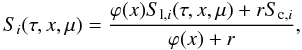
2. Governing equations
The atmosphere is assumed to be plane-parallel, the primary source of photons to be of thermal origin, the incident radiation to be either zero or axisymmetric, and the magnetic field to be zero or micro-turbulent. These assumptions imply that the radiation field is cylindrically symmetric and can be described by the two Stokes parameters I and Q, if one chooses the reference direction for the measurement of Q such that positive Q is perpendicular to the surface of the atmosphere. Because of the cylindrical symmetry Stokes U = 0.
The polarized transfer equation for the Stokes parameters I and
Q can be written in a component form as ![Mathematical equation: \begin{equation} \mu {\partial I_i \over \partial \tau} = \left[\varphi(x)+r\right] \left[I_i(\tau,x,\mu)-S_i(\tau,x,\mu)\right], \quad i=0,1, \label{rte_stokes_component} \end{equation}](/articles/aa/full_html/2011/03/aa15813-10/aa15813-10-eq10.png) (1)where
μ = cosθ, with θ being the co-latitude
with respect to the atmospheric normal, τ the line optical depth defined by
dτ = −kldz, with
kl the frequency-averaged line absorption coefficient, and
ϕ(x) the normalized Voigt function. The
frequency x is measured in units of the Doppler width, assumed to be
constant, with x = 0 at line center. The ratio of continuum to line
absorption coefficient is denoted by r. The total source vector is given by
(1)where
μ = cosθ, with θ being the co-latitude
with respect to the atmospheric normal, τ the line optical depth defined by
dτ = −kldz, with
kl the frequency-averaged line absorption coefficient, and
ϕ(x) the normalized Voigt function. The
frequency x is measured in units of the Doppler width, assumed to be
constant, with x = 0 at line center. The ratio of continuum to line
absorption coefficient is denoted by r. The total source vector is given by
 (2)where
Sc,i are the components of the unpolarized
continuum source vector. We assume that
Sc,0 = B, where B is the
Planck function at line center, and Sc,1 = 0. The line source
vector can be written as
(2)where
Sc,i are the components of the unpolarized
continuum source vector. We assume that
Sc,0 = B, where B is the
Planck function at line center, and Sc,1 = 0. The line source
vector can be written as 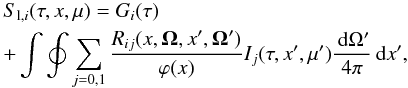 (3)where
dΩ′ = sinθ′ dθ′ dχ′. The outgoing
and incoming ray directions Ω and Ω′ are
defined, respectively, by their polar angles (θ,χ) and
(θ′,χ′). For simplicity, we assume that the primary
source is unpolarized, namely that only G0(τ)
is non-zero. It is proportional to the Planck function at line center. The term
Rij(x,Ω,x′,Ω′)
denote the elements of the redistribution matrix for Rayleigh scattering (Domke & Hubeny 1988; Bommier 1997a).
(3)where
dΩ′ = sinθ′ dθ′ dχ′. The outgoing
and incoming ray directions Ω and Ω′ are
defined, respectively, by their polar angles (θ,χ) and
(θ′,χ′). For simplicity, we assume that the primary
source is unpolarized, namely that only G0(τ)
is non-zero. It is proportional to the Planck function at line center. The term
Rij(x,Ω,x′,Ω′)
denote the elements of the redistribution matrix for Rayleigh scattering (Domke & Hubeny 1988; Bommier 1997a).
According to the decomposition technique described in HF10, we can write
Ii and
Sl,i as 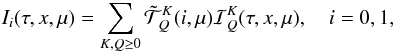 (4)
(4)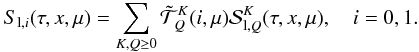 (5)We have four terms
in the summation over K and Q corresponding to
K = Q = 0, K = 2 with
Q = 0,1,2. The irreducible tensors
(5)We have four terms
in the summation over K and Q corresponding to
K = Q = 0, K = 2 with
Q = 0,1,2. The irreducible tensors
 are defined in HF10. An
explicit expression of Eq. (4) can be found
in Eq. (42). The total source vector
Si has a decomposition similar to Eq. (5). The irreducible line source vector components
are defined in HF10. An
explicit expression of Eq. (4) can be found
in Eq. (42). The total source vector
Si has a decomposition similar to Eq. (5). The irreducible line source vector components
 may be written as
 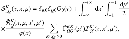 (6)where
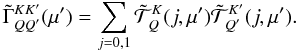 (7)The coefficients
 are given in the Appendix of
HF10. The functions
are given in the Appendix of
HF10. The functions  in Eq. (6) take the form
 ![Mathematical equation: \begin{equation} {\tilde{\mathcal R}}^0_0=\alpha \tilde r^{(0)}_{\rm II} + \left[\beta^{(0)}-\alpha\right] \tilde r^{(0)}_{\rm III}, \label{R00} \end{equation}](/articles/aa/full_html/2011/03/aa15813-10/aa15813-10-eq48.png) (8)
(8)![Mathematical equation: \begin{equation} {\tilde{\mathcal R}}^2_Q=W_2\mu_2\left\{\alpha \tilde r^{(Q)}_{\rm II} + \left[\beta^{(2)}-\alpha\right] \tilde r^{(Q)}_{\rm III}\right\}, \quad Q=0,1,2, \label{R2Q} \end{equation}](/articles/aa/full_html/2011/03/aa15813-10/aa15813-10-eq49.png) (9)where
W2(Jl,Ju)
is an atomic depolarization factor depending on the angular momentum of the lower and upper
levels of the transition. The coefficients α and
β(K) (Bommier 1997b) are branching ratios
(9)where
W2(Jl,Ju)
is an atomic depolarization factor depending on the angular momentum of the lower and upper
levels of the transition. The coefficients α and
β(K) (Bommier 1997b) are branching ratios
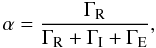 (10)and
 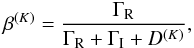 (11)where ΓR is the
radiative rate, ΓI and ΓE the inelastic and elastic collisional rates,
and D(K) the collisional depolarization rate
such that D(0) = 0. The coefficient
μ2 takes the effects of a micro-turbulent magnetic field into
account. It depends on the magnetic field probability density function (see e.g., Landi Degl’Innocenti & Landolfi 2004, p. 215) and
is unity in the absence of magnetic fields. Since the Hanle effect acts only in the line
core, the coefficient μ2 should be set to unity outside the line
core. The
(11)where ΓR is the
radiative rate, ΓI and ΓE the inelastic and elastic collisional rates,
and D(K) the collisional depolarization rate
such that D(0) = 0. The coefficient
μ2 takes the effects of a micro-turbulent magnetic field into
account. It depends on the magnetic field probability density function (see e.g., Landi Degl’Innocenti & Landolfi 2004, p. 215) and
is unity in the absence of magnetic fields. Since the Hanle effect acts only in the line
core, the coefficient μ2 should be set to unity outside the line
core. The  (with X = II or III) are the azimuthal Fourier coefficients of order 0, 1, and 2 of Hummer (1962)’s PRD functions
rII and rIII. They are defined by
(with X = II or III) are the azimuthal Fourier coefficients of order 0, 1, and 2 of Hummer (1962)’s PRD functions
rII and rIII. They are defined by
![Mathematical equation: \begin{eqnarray} &&\tilde r^{(Q)}_{\rm X}(x,\mu,x^{\prime},\mu^{\prime}) = {2-\delta_{0Q} \over 2\pi} \nonumber \\ \label{tilderq} && \quad \times \int_0^{2\pi} r_{\rm X}(x,\mu,x^{\prime},\mu^{\prime},\chi-\chi^{\prime}) \cos [Q(\chi-\chi^{\prime})] \md(\chi-\chi^{\prime}). \end{eqnarray}](/articles/aa/full_html/2011/03/aa15813-10/aa15813-10-eq68.png) (12)The
components
(12)The
components  satisfy a transfer
equation similar to Eq. (1). The source term
is given by Eq. (2), where
Sl,i and
Sc,i are replaced by
satisfy a transfer
equation similar to Eq. (1). The source term
is given by Eq. (2), where
Sl,i and
Sc,i are replaced by
 and
and
 .
Introducing the four-component vectors
.
Introducing the four-component vectors  and
and
 , we can re-write
Eq. (6) in vector form as
, we can re-write
Eq. (6) in vector form as  (13)The
primary source vector is
(13)The
primary source vector is  ,
where G0(τ) = ϵB with
ϵ = ΓI/(ΓI + ΓR). The (4 × 4) matrix
,
where G0(τ) = ϵB with
ϵ = ΓI/(ΓI + ΓR). The (4 × 4) matrix
 is diagonal, i.e.,
 ![Mathematical equation: \hbox{${\tilde{\bm{\mathcal R}}}={\rm diag}\left[\tilde {\mathcal R}^{0}_{0}, \tilde{\mathcal R}^{2}_{0},\tilde{\mathcal R}^{2}_{1},\tilde{\mathcal R}^{2}_{2}\right]$}](/articles/aa/full_html/2011/03/aa15813-10/aa15813-10-eq79.png) .
Its elements are defined in Eqs. (8) and
(9). The (4 × 4) matrix
Γ is a full matrix with elements
.
Its elements are defined in Eqs. (8) and
(9). The (4 × 4) matrix
Γ is a full matrix with elements
 .
Owing to its symmetry, it has only ten independent elements (see Eq. (7) and also HF10). When
is independent of μ and μ′ (CRD or angle-averaged PRD),
only the two components of the source vector corresponding to the index
Q = 0 are non-zero. In this case, one recovers the usual Rayleigh
scattering whereby the radiation field and source vector are fully described by
two-component vectors.
.
Owing to its symmetry, it has only ten independent elements (see Eq. (7) and also HF10). When
is independent of μ and μ′ (CRD or angle-averaged PRD),
only the two components of the source vector corresponding to the index
Q = 0 are non-zero. In this case, one recovers the usual Rayleigh
scattering whereby the radiation field and source vector are fully described by
two-component vectors.
3. Numerical methods of solution
We present three iterative methods to solve the problem of angle-dependent PRD. The first two are ALI type methods and the third is a scattering expansion method. We assume a plane-parallel slab geometry with a given total optical thickness.
3.1. The polarized accelerated lambda iteration approaches
For notational simplicity, we neglect the explicit dependence of
ℐ and  on τ. The dependence on x and μ
appear as subscripts. The formal solution of the transfer equation for the four-component
irreducible vector ℐ can be written as
on τ. The dependence on x and μ
appear as subscripts. The formal solution of the transfer equation for the four-component
irreducible vector ℐ can be written as ![Mathematical equation: \begin{equation} {\bm{\mathcal I}}_{x\mu} = {\bf \Lambda}_{x\mu} \left[{\bm{\mathcal S}}_{x\mu} \right] + {\bm T}_{x\mu}, \label{formal_solution} \end{equation}](/articles/aa/full_html/2011/03/aa15813-10/aa15813-10-eq87.png) (14)where
Txμ is the directly
transmitted part of the intensity vector and
Λxμ is the frequency- and
angle-dependent (4 × 4) integral operator. We introduce the operator splitting written as
(14)where
Txμ is the directly
transmitted part of the intensity vector and
Λxμ is the frequency- and
angle-dependent (4 × 4) integral operator. We introduce the operator splitting written as
 (15)where
 is the
diagonal approximate operator (see Olson et al.
1986). We now write the total source vector
is the
diagonal approximate operator (see Olson et al.
1986). We now write the total source vector
 and the line source vector
  as
as  (16)where
n is the iteration index. Combining Eqs. (15) and (16) with
Eq. (13), we derive an equation for the
line source vector corrections that can be written as
(16)where
n is the iteration index. Combining Eqs. (15) and (16) with
Eq. (13), we derive an equation for the
line source vector corrections that can be written as ![Mathematical equation: \begin{eqnarray} && \delta{\bm{\mathcal S}}^n_{{\rm l},x\mu} - \int_{-\infty}^{+\infty} \int_{-1}^{+1} {\tilde{\bm{\mathcal R}}_{x\mu,x^{\prime}\mu^{\prime}} \over \varphi_x} {\bf \Gamma}_{\mu^{\prime}} p_{x^{\prime}}\nonumber \\ \label{source_corrections} && \times {\bf \Lambda}^\ast_{x^{\prime}\mu^{\prime}} \left[\delta{\bm{\mathcal S}}^n_{{\rm l},x^{\prime}\mu^{\prime}}\right] {\md\mu^{\prime} \over 2} \md x^{\prime} = {\bm{\mathcal G}}(\tau) + \overline {\bm{\mathcal J}}^{\,n}_{x\mu}-{\bm{\mathcal S}}^n_{{\rm l},x\mu}, \end{eqnarray}](/articles/aa/full_html/2011/03/aa15813-10/aa15813-10-eq96.png) (17)where
px = ϕx/(ϕx + r)
and
(17)where
px = ϕx/(ϕx + r)
and ![Mathematical equation: \begin{equation} \overline {\bm{\mathcal J}}^{\,n}_{x\mu} = \int_{-\infty}^{+\infty} \int_{-1}^{+1}{\tilde{\bm{\mathcal R}}_{x\mu,x^{\prime}\mu^{\prime}} \over \varphi_x} {\bf \Gamma}_{\mu^{\prime}}{\bf \Lambda}_{x^{\prime}\mu^{\prime}} \left[{\bm{\mathcal S}}^n_{x^{\prime}\mu^{\prime}}\right] {\md\mu^{\prime} \over 2} \md x^{\prime}. \label{jvector} \end{equation}](/articles/aa/full_html/2011/03/aa15813-10/aa15813-10-eq98.png) (18)For this investigation,
we chose the Jacobi decomposition of the Λ operator. Superior
iterative methods such as the Gauss-Seidel (GS) and the successive overrelaxation (SOR)
technique were introduced into scalar radiative transfer theory by Trujillo Bueno & Fabiani Bendicho (1995). These methods provide
faster convergence rates than the Jacobi method. Trujillo
Bueno & Manso Sainz (1999) extended these methods to the case of
resonance scattering. The generalization to the Hanle effect was developed by Manso Sainz & Trujillo Bueno (1999). In these
references, CRD is assumed for the frequency redistribution. The GS and SOR methods were
extended to the case of angle-averaged PRD in Sampoorna
& Trujillo Bueno (2010). In this first attempt at developing ALI methods
for angle-dependent PRD functions, we chose the simpler Jacobi decomposition. We now
describe two different methods of solution for Eq. (17).
(18)For this investigation,
we chose the Jacobi decomposition of the Λ operator. Superior
iterative methods such as the Gauss-Seidel (GS) and the successive overrelaxation (SOR)
technique were introduced into scalar radiative transfer theory by Trujillo Bueno & Fabiani Bendicho (1995). These methods provide
faster convergence rates than the Jacobi method. Trujillo
Bueno & Manso Sainz (1999) extended these methods to the case of
resonance scattering. The generalization to the Hanle effect was developed by Manso Sainz & Trujillo Bueno (1999). In these
references, CRD is assumed for the frequency redistribution. The GS and SOR methods were
extended to the case of angle-averaged PRD in Sampoorna
& Trujillo Bueno (2010). In this first attempt at developing ALI methods
for angle-dependent PRD functions, we chose the simpler Jacobi decomposition. We now
describe two different methods of solution for Eq. (17).
3.1.1. Frequency-angle by frequency-angle (FABFA) method
This FABFA method is a generalization of the FBF method introduced by Paletou & Auer (1995). In matrix form,
Eq. (17) can be written as
 (19)where the
residual vector rn is given by
the right-hand side of Eq. (17). At each
depth point, rn and
(19)where the
residual vector rn is given by
the right-hand side of Eq. (17). At each
depth point, rn and
 are vectors of
length
4Nx 2Nμ,
where Nx is the number of frequency points
in the range [0,xmax] 2 and Nμ is the number of angle
points in the range [0 < μ ≤ 1] . The matrix
A thus has dimensions
(4Nx 2Nμ × 4Nx 2Nμ).
For a given x, x′, μ, and
μ′, the matrix A can be decomposed into
(Nx 2Nμ × Nx 2Nμ)
blocks of 4 × 4 elements. In each block, denoted by
are vectors of
length
4Nx 2Nμ,
where Nx is the number of frequency points
in the range [0,xmax] 2 and Nμ is the number of angle
points in the range [0 < μ ≤ 1] . The matrix
A thus has dimensions
(4Nx 2Nμ × 4Nx 2Nμ).
For a given x, x′, μ, and
μ′, the matrix A can be decomposed into
(Nx 2Nμ × Nx 2Nμ)
blocks of 4 × 4 elements. In each block, denoted by
 ,
the elements may be written as
,
the elements may be written as  (20)where
m = 1,...,Nx,
n = 1,...,Nx′,
α = 1,...,2Nμ,
and
β = 1,...,2Nμ′,
and E is the identity operator. The coefficients
wβ denote the μ′
integration weights and gmα,nβ are
defined by
(20)where
m = 1,...,Nx,
n = 1,...,Nx′,
α = 1,...,2Nμ,
and
β = 1,...,2Nμ′,
and E is the identity operator. The coefficients
wβ denote the μ′
integration weights and gmα,nβ are
defined by  (21)where
 are the frequency (x′) integration weights. The FABFA method requires
the calculation of the matrix A-1 before the
iteration cycle.
are the frequency (x′) integration weights. The FABFA method requires
the calculation of the matrix A-1 before the
iteration cycle.
3.1.2. The core-wing separation method for angle-dependent PRD
Here we describe a generalization of the core-wing method of Paletou & Auer (1995). According to the ALI methods, the
right-hand side of Eq. (17) must be
calculated as accurately as possible but in the left-hand side there is some flexibility
in the choice of the operator acting on the corrections
 . The choice
of this operator affects the speed of convergence of the process but not the final
solution. For Rayleigh scattering, we already know that the angle-dependence of the PRD
functions has only a mild effect on the Q/I
profiles. Hence, in the matrix
. The choice
of this operator affects the speed of convergence of the process but not the final
solution. For Rayleigh scattering, we already know that the angle-dependence of the PRD
functions has only a mild effect on the Q/I
profiles. Hence, in the matrix  in the left-hand side, we retain the two terms corresponding to the index
Q = 0 and set to zero the two other terms corresponding to
Q = 1 and Q = 2. This is equivalent to making the
approximation
in the left-hand side, we retain the two terms corresponding to the index
Q = 0 and set to zero the two other terms corresponding to
Q = 1 and Q = 2. This is equivalent to making the
approximation  (22)where ℰ and
 are (4 × 4)
diagonal matrices defined by ℰ = diag [1,1,0,0] and
are (4 × 4)
diagonal matrices defined by ℰ = diag [1,1,0,0] and
![Mathematical equation: \hbox{${\bm{\mathcal R}}^{\rm AA}_{xx^{\prime}}={\rm diag}\left[ \left({\mathcal R}^{\rm AA}_{xx^{\prime}}\right)^0_0, \left({\mathcal R}^{\rm AA}_{xx^{\prime}}\right)^2_0, 0,0\right]$}](/articles/aa/full_html/2011/03/aa15813-10/aa15813-10-eq136.png) ,
with
,
with ![Mathematical equation: \begin{equation} \left({\mathcal R}^{\rm AA}_{xx^{\prime}}\right)^0_0=\alpha r^{\rm II-AA}_{xx^{\prime}} + \left[\beta^{(0)}-\alpha\right] r^{\rm III-AA}_{xx^{\prime}}, \label{R00-crdcs} \end{equation}](/articles/aa/full_html/2011/03/aa15813-10/aa15813-10-eq137.png) (23)
(23)![Mathematical equation: \begin{equation} \left({\mathcal R}^{\rm AA}_{xx^{\prime}}\right)^2_0=W_2\mu_2 \left\{\alpha r^{\rm II-AA}_{xx^{\prime}} + \left[\beta^{(2)}-\alpha\right] r^{\rm III-AA}_{xx^{\prime}}\right\}, \label{R2Q-crdcs} \end{equation}](/articles/aa/full_html/2011/03/aa15813-10/aa15813-10-eq138.png) (24)and
(24)and
 and
and  are the type-II and type-III angle-averaged (AA) redistribution functions. By comparing
with the FABFA method, we find that this approximation leads to a correct converged
solution, but at a much less computational cost (see Sect. 5).
are the type-II and type-III angle-averaged (AA) redistribution functions. By comparing
with the FABFA method, we find that this approximation leads to a correct converged
solution, but at a much less computational cost (see Sect. 5).
Substituting Eq. (22) in Eq. (17), we obtain ![Mathematical equation: \begin{eqnarray} & & \delta{\bm{\mathcal S}}^n_{{\rm l},x\mu} - \nonumber\\ \label{source_corrections-crdcs} && \!\!\!\!\int_{-\infty}^{+\infty} {\bm{\mathcal R}^{\rm AA}_{xx^{\prime}} \over \varphi_x}\!\int_{-1}^{+1} {\bf{\mathcal E}} {\bf \Gamma}_{\mu^{\prime}} p_{x^{\prime}}{\bf \Lambda}^\ast_{x^{\prime}\mu^{\prime}} \left[\delta{\bm{\mathcal S}}^n_{{\rm l},x^{\prime}\mu^{\prime}}\right] {\md\mu^{\prime} \over 2} \md x^{\prime} = {\bm{ r}}^{n}_{x\mu}. \end{eqnarray}](/articles/aa/full_html/2011/03/aa15813-10/aa15813-10-eq141.png) (25)To
the above equation, we now apply the core-wing method (Paletou & Auer 1995; Nagendra et al.
1999; Fluri et al. 2003), namely
(25)To
the above equation, we now apply the core-wing method (Paletou & Auer 1995; Nagendra et al.
1999; Fluri et al. 2003), namely
 (26)
(26) (27)where
xc is the frequency that distinguishes the line core and
the wing. A value of xc = 3.5 Doppler widths for the
separation frequency is a reasonable choice. Combining Eqs. (26) and (27) with Eq. (25),
we obtain the expression for the line source vector corrections
(27)where
xc is the frequency that distinguishes the line core and
the wing. A value of xc = 3.5 Doppler widths for the
separation frequency is a reasonable choice. Combining Eqs. (26) and (27) with Eq. (25),
we obtain the expression for the line source vector corrections  (28)where
![Mathematical equation: \hbox{${\mathcal W}={\rm diag}[1, W_2\mu_2, W_2\mu_2, W_2\mu_2]$}](/articles/aa/full_html/2011/03/aa15813-10/aa15813-10-eq147.png) and
and ![Mathematical equation: \hbox{${\bf{\mathcal B}}={\rm diag}\left[\beta^{(0)},\beta^{(2)},\beta^{(2)}, \beta^{(2)}\right]$}](/articles/aa/full_html/2011/03/aa15813-10/aa15813-10-eq148.png) . The
frequency and angle-independent four-dimensional vector
ΔTcore is given by
. The
frequency and angle-independent four-dimensional vector
ΔTcore is given by
![Mathematical equation: \begin{equation} {\bm {\Delta T}}^{\rm core} = \int_{-x_{\rm c}}^{+x_{\rm c}} \varphi_{x^{\prime}} \int_{-1}^{+1} p_{x^{\prime}}{\bf \Gamma}_{\mu^{\prime}} {\bf \Lambda}^\ast_{x^{\prime}\mu^{\prime}} \left[\delta{\bm{\mathcal S}}^n_{{\rm l},x^{\prime}\mu^{\prime}}\right] {\md\mu^{\prime} \over 2} \md x^{\prime}, \label{deltatcore} \end{equation}](/articles/aa/full_html/2011/03/aa15813-10/aa15813-10-eq150.png) (29)and the
frequency-dependent but angle-independent four-dimensional vector
(29)and the
frequency-dependent but angle-independent four-dimensional vector
 is given
by
is given
by ![Mathematical equation: \begin{equation} {\bm {\Delta T}}^{\rm wing}_x = \int_{-1}^{+1} p_{x}{\bf \Gamma}_{\mu^{\prime}} {\bf \Lambda}^\ast_{x\mu^{\prime}} \left[\delta{\bm{\mathcal S}}^n_{{\rm l},x\mu^{\prime}}\right] {\md\mu^{\prime} \over 2}\cdot \label{deltatwing} \end{equation}](/articles/aa/full_html/2011/03/aa15813-10/aa15813-10-eq152.png) (30)In Eq. (28),
αx is the core-wing separation
coefficient. In the core αx = 0 and in the
wings
(30)In Eq. (28),
αx is the core-wing separation
coefficient. In the core αx = 0 and in the
wings  .
.
To evaluate ΔTcore,
we consider Eq. (28) with
αx = 0 and apply the operator
![Mathematical equation: \hbox{$\int_{-x_{\rm c}}^{+x_{\rm c}} \varphi_{x}\int_{-1}^{+1} p_{x}{\bf \Gamma}_{\mu} {\bf \Lambda}^\ast_{x\mu}[\,]{\md\mu \over 2} \md x$}](/articles/aa/full_html/2011/03/aa15813-10/aa15813-10-eq156.png) from left. After some algebra,
we obtain
from left. After some algebra,
we obtain ![Mathematical equation: \begin{eqnarray} & & {\bm {\Delta T}}^{\rm core} = \nonumber\\ \label{deltatcore-eval}& & \left[{\bf E} - \left(\int_{-x_{\rm c}}^{+x_{\rm c}} \varphi_{x}\int_{-1}^{+1} p_{x}{\bf \Gamma}_{\mu} {\bf \Lambda}^\ast_{x\mu}{{\rm d}\mu \over 2} {\rm d}x\right) \, {\mathcal W}{{\mathcal B}} {{\mathcal E}}\right]^{-1} {\overline {\bm{ r}}}^{\,n}, \end{eqnarray}](/articles/aa/full_html/2011/03/aa15813-10/aa15813-10-eq157.png) (31)where
(31)where
![Mathematical equation: \begin{equation} {\overline {\bm r}}^n=\int_{-x_{\rm c}}^{+x_{\rm c}} \varphi_{x}\int_{-1}^{+1} p_{x} {\bf \Gamma}_{\mu}{\bf \Lambda}^\ast_{x\mu}\left[{\bm{ r}}^n_{x\mu} \right]{\md\mu \over 2} \md x. \label{rbarn} \end{equation}](/articles/aa/full_html/2011/03/aa15813-10/aa15813-10-eq158.png) (32)Similarly, to evaluate
we apply
the operator
(32)Similarly, to evaluate
we apply
the operator ![Mathematical equation: \hbox{$\int_{-1}^{+1} p_{x}{\bf \Gamma}_{\mu}{\bf \Lambda}^\ast_{x\mu}[\,]{\md\mu \over 2}$}](/articles/aa/full_html/2011/03/aa15813-10/aa15813-10-eq159.png) from the left to Eq. (28), to obtain
from the left to Eq. (28), to obtain
![Mathematical equation: \begin{eqnarray} &&\!\!\!{\bm {\Delta T}}^{\rm wing}_x = \left[{\bf E} -\alpha_x\alpha\left(\int_{-1}^{+1} p_{x}{\bf \Gamma}_{\mu} {\bf \Lambda}^\ast_{x\mu}{\md\mu \over 2}\right) \, {\mathcal W}{{\mathcal E}}\right]^{-1} \nonumber \\ && \label{deltatwing-eval} \!\!\!\!\!\!\!\times \left[{\tilde {\bm{ r}}}^{n}_x + (1-\alpha_x)p_x \left(\int_{-1}^{+1} {\bf \Gamma}_{\mu}{\bf \Lambda}^\ast_{x\mu}{\md\mu \over 2}\right){\mathcal W}{{\mathcal B}}{{\mathcal E}}\,{\bm {\Delta T}}^{\rm core}\right], \end{eqnarray}](/articles/aa/full_html/2011/03/aa15813-10/aa15813-10-eq160.png) (33)where
(33)where
![Mathematical equation: \begin{equation} {\tilde {\bm{ r}}}^{n}_x = \int_{-1}^{+1} p_x {\bf \Gamma}_{\mu}{\bf \Lambda}^\ast_{x\mu}\left[{\bm{ r}}^n_{x\mu} \right]{\md\mu \over 2}\cdot \label{rtilde} \end{equation}](/articles/aa/full_html/2011/03/aa15813-10/aa15813-10-eq161.png) (34)The equations for
and
ΔTcore are then
incorporated into Eq. (28) to calculate
the corrections to the source vector.
(34)The equations for
and
ΔTcore are then
incorporated into Eq. (28) to calculate
the corrections to the source vector.
3.2. Scattering expansion approach
We present an iterative method of a different type that can also be used with an angle-dependent PRD. It is based on a Neumann series expansion of the components of the source vector contributing to the polarization. This Neumann series amounts to an expansion in the mean number of scattering events (see Frisch et al. 2009). Its first term yields the so-called single scattering solution. For Rayleigh scattering with an angle-dependent PRD, the single scattering solution is given in Eq. (25) of HF10. Here, following Frisch et al. (2009), we include higher order terms. The main steps of this method are given below.
We first neglect polarization in the calculation of Stokes I, i.e., we
assume that Stokes I is given by the component
 . This
component is the solution of a non-LTE unpolarized radiative transfer equation. We
calculate it with a scalar version of the core-wing ALI method described in Sect. 3.1.2, using
. This
component is the solution of a non-LTE unpolarized radiative transfer equation. We
calculate it with a scalar version of the core-wing ALI method described in Sect. 3.1.2, using  as a PRD
function. Knowing , we can
calculate the single scattering approximation for each component
as a PRD
function. Knowing , we can
calculate the single scattering approximation for each component
 (Q = 0,1,2). It may be written as
 ![Mathematical equation: \begin{eqnarray} &&\left[\tilde{\mathcal S}^2_{{\rm l},Q}\right]^{(1)}(\tau,x,\mu)= \nonumber\\ \label{approximation_s2q_ss} & &\!\!\! \int_{-\infty}^{+\infty}\!\!\!\int_{-1}^{+1} \frac{ \tilde R^2_{Q}(x,\mu,x',\mu')}{\varphi(x)} \tilde \Gamma_{Q0}^{20}(\mu'){\mathcal I}^{0}_{0}(\tau,x',\mu')\,\frac{{\md}\mu'}{2}{\md}x'. \end{eqnarray}](/articles/aa/full_html/2011/03/aa15813-10/aa15813-10-eq165.png) (35)The
superscript 1 stands for single scattering. The corresponding radiation field
(35)The
superscript 1 stands for single scattering. The corresponding radiation field
![Mathematical equation: \hbox{$\left[\tilde{\mathcal I}^2_Q\right]^{(1)}$}](/articles/aa/full_html/2011/03/aa15813-10/aa15813-10-eq166.png) is
calculated with a formal solver and it serves as a starting point for calculating the
higher order terms. For order (n),
is
calculated with a formal solver and it serves as a starting point for calculating the
higher order terms. For order (n), ![Mathematical equation: \begin{eqnarray} &&\left[\tilde{\mathcal S}^2_{{\rm l},Q}\right]^{(n)}= \left[\tilde{\mathcal S}^2_{{\rm l},Q}\right]^{(1)} + \int_{-\infty}^{+\infty}\md x^{\prime}\int_{-1}^{+1} {\md\mu^{\prime} \over 2} \nonumber \\ \label{approximation_s2q_ms}&& \times{\tilde {\mathcal R}^{2}_{Q}(x,\mu,x^{\prime},\mu^{\prime}) \over \varphi(x)} \sum_{Q^{\prime} \ge 0} \tilde{\Gamma}^{22}_{QQ^{\prime}}(\mu^{\prime}) \left[\tilde{\mathcal I}^{2}_{Q^{\prime}}\right]^{(n-1)} (\tau,x^{\prime},\mu^{\prime}). \end{eqnarray}](/articles/aa/full_html/2011/03/aa15813-10/aa15813-10-eq168.png) (36)The
iteration is continued until a convergence criterion defined in Sect. 5 is satisfied. The component is calculated
only once. We emphasize that this method will be reliable only if the polarization rate
remains small, say smaller than 20%.
(36)The
iteration is continued until a convergence criterion defined in Sect. 5 is satisfied. The component is calculated
only once. We emphasize that this method will be reliable only if the polarization rate
remains small, say smaller than 20%.
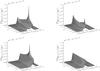 |
Fig. 1 Surface plots of azimuth averaged redistribution functions of type II (left panels) and of type III (right panels) with Q = 0. The X-axis represents the outgoing frequency x, and the Y-axis represents outgoing direction μ. The incoming direction is μ′ = 0.3. The damping parameter a = 0.001. The top two panels correspond to the incoming frequency x′ = 3, and the bottom panels to x′ = 4. |
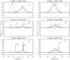 |
Fig. 2 Azimuth averaged redistribution functions of type II (left panels) and of type III (right panels), plotted as a function of the outgoing frequency x, for different choices of μ, and μ′. The damping parameter a = 0.001. Thin lines correspond to x′ = 1 and thick lines to x′ = 4. Solid, dotted and dashed lines correspond respectively to Q = 0,1, and 2. |
4. The Fourier azimuthal averages and coefficients of the PRD functions
The numerical methods described in the preceding section involve the azimuthal Fourier
coefficients  and
and
 for
Q = 0,1,2 defined in Eq. (12). The azimuthal averages with Q = 0 were considered in the
classical work by Milkey et al. (1975). Subsequently
Vardavas (1976), Faurobert (1987), and Wallace & Yelle
(1989) devised methods to evaluate various azimuthal moments of the angle-dependent
frequency redistribution functions. We stress that the moments of order
Q = 0 are normalized to the absorption profile when integrated over all the
incoming frequencies and angles, while the moments of orders Q = 1 and
Q = 2 are normalized to zero. For reasons that we explain below, these
normalizations should be satisfied to great accuracy.
for
Q = 0,1,2 defined in Eq. (12). The azimuthal averages with Q = 0 were considered in the
classical work by Milkey et al. (1975). Subsequently
Vardavas (1976), Faurobert (1987), and Wallace & Yelle
(1989) devised methods to evaluate various azimuthal moments of the angle-dependent
frequency redistribution functions. We stress that the moments of order
Q = 0 are normalized to the absorption profile when integrated over all the
incoming frequencies and angles, while the moments of orders Q = 1 and
Q = 2 are normalized to zero. For reasons that we explain below, these
normalizations should be satisfied to great accuracy.
Here, we use a 31-point Gauss-Legendre quadrature to perform the integration over (χ − χ′). Since rX(x,μ,x′,μ′,χ − χ′) (X = II and III) are even functions of (χ − χ′), the integration can be limited to the range 0 ≤ (χ − χ′) ≤ π.
In Fig. 1, we show surface plots of
 and
and
 (left panels and right panels,
respectively) as a function of the scattered frequency x and the scattered
direction μ for the incoming frequencies x′ = 3 and
x′ = 4, and the incoming direction μ′ = 0.3. The damping
parameter a of the Voigt profile
ϕx is taken to be equal to 0.001. The
behaviors at x′ = 3 and x′ = 4 are typical of line core
and line wings, respectively. We can observe that the functions
(left panels and right panels,
respectively) as a function of the scattered frequency x and the scattered
direction μ for the incoming frequencies x′ = 3 and
x′ = 4, and the incoming direction μ′ = 0.3. The damping
parameter a of the Voigt profile
ϕx is taken to be equal to 0.001. The
behaviors at x′ = 3 and x′ = 4 are typical of line core
and line wings, respectively. We can observe that the functions
 and
and
 have
similar behaviors for x′ = 3 but quite different ones for
x′ = 4. For the wing frequency x′ = 4, one recovers
features that are typical of the angle-averaged PRD functions, namely
as a
function of x is peaked at the incident frequency x′,
while
shows a CRD–type behavior with a single peak at x = 0 for all values of
μ. The results shown for μ′ = 0.3 hold for all incoming
directions 0 < μ′ < 1.
have
similar behaviors for x′ = 3 but quite different ones for
x′ = 4. For the wing frequency x′ = 4, one recovers
features that are typical of the angle-averaged PRD functions, namely
as a
function of x is peaked at the incident frequency x′,
while
shows a CRD–type behavior with a single peak at x = 0 for all values of
μ. The results shown for μ′ = 0.3 hold for all incoming
directions 0 < μ′ < 1.
Figure 2 shows  and
and
 for
all the three values Q = 0,1,2 as a function of the outgoing frequency
x for different choices of (μ, μ′) and
different incoming frequencies x′. Our choice of
(μ,μ′) values for Fig. 2 are identical to those of Wallace &
Yelle (1989) in their analysis of the azimuth-averaged type II redistribution
function. The frequencies x′ = 1 and x′ = 4 are
representative of the line center and wing behaviors, respectively. Figure 2 clearly shows that the sharp peaks appearing in
Fig. 1 for Q = 0 also exist for
Q = 1,2 for forward and backward scattering (see panels b, c, e, f).
Actually, surface plots for Q = 1,2 are very similar to the surface plots
shown in Fig. 1. However, because they are normalized
to zero,
for
all the three values Q = 0,1,2 as a function of the outgoing frequency
x for different choices of (μ, μ′) and
different incoming frequencies x′. Our choice of
(μ,μ′) values for Fig. 2 are identical to those of Wallace &
Yelle (1989) in their analysis of the azimuth-averaged type II redistribution
function. The frequencies x′ = 1 and x′ = 4 are
representative of the line center and wing behaviors, respectively. Figure 2 clearly shows that the sharp peaks appearing in
Fig. 1 for Q = 0 also exist for
Q = 1,2 for forward and backward scattering (see panels b, c, e, f).
Actually, surface plots for Q = 1,2 are very similar to the surface plots
shown in Fig. 1. However, because they are normalized
to zero,  and
and
 for
Q = 1,2 can take negative values as can be observed in Fig. 2. In the upper panels of this figure, one can observe that
the coefficients
decrease in magnitude with increasing Q. This result agrees with the curves
shown by Domke & Hubeny (1988) for
μ = 0.8 and μ′ = 0.2 (see their Fig. 3). However, for
the special cases of forward and backward scattering (panels b, c, e, f), the Fourier
coefficients for Q = 1 and 2 can become larger than the
Q = 0 coefficients.
for
Q = 1,2 can take negative values as can be observed in Fig. 2. In the upper panels of this figure, one can observe that
the coefficients
decrease in magnitude with increasing Q. This result agrees with the curves
shown by Domke & Hubeny (1988) for
μ = 0.8 and μ′ = 0.2 (see their Fig. 3). However, for
the special cases of forward and backward scattering (panels b, c, e, f), the Fourier
coefficients for Q = 1 and 2 can become larger than the
Q = 0 coefficients.
A significant difference between angle-averaged and angle-dependent PRD functions is the
presence of very sharp and narrow peaks for x ≃ x′ and
μ ≃ μ′ for the angle-dependent PRD functions. This has
important implications for the numerical evaluation of the scattering integrals (see
Eq. (6)). It is well known in scalar
non-LTE radiative transfer calculations that an accurate normalization is required for the
profile function and the PRD functions, especially for lines with a large optical thickness
and a very small thermalization parameter. Any error will indeed act as a spurious sink or
source of photons. To achieve the normalization to a high accuracy, a very fine frequency
grid is needed. However, the use of such fine frequency grids in the transfer calculations
require large computing resources. Hence, strategies have been developed in the past (see
for e.g., Wallace & Yelle 1989) to handle
frequency quadratures in angle-dependent PRD problems. For unpolarized transfer problems,
Adams et al. (1971) proposed a natural cubic spline
representation for the radiation field. In this paper, we have developed our own strategy to
maintain the computational cost of the radiative transfer calculations at a reasonable level
while ensuring a high accuracy:  is
normalized to ϕx with an accuracy of 99% and
the integrals of ,
Q = 1,2, over incoming frequencies and directions are around
10-7.
is
normalized to ϕx with an accuracy of 99% and
the integrals of ,
Q = 1,2, over incoming frequencies and directions are around
10-7.
We first start with a frequency grid typical of PRD line transfer problems on which the
transfer equation will be solved. The choice of the actual frequency grid is given below in
Sect. 5. We then sub-divide each frequency interval
into a fine mesh of Simpson quadrature points (e.g., 41-point Simpson formula) on which we
calculate the coefficients  . A
seven-point Gaussian quadrature formula with μ in the range
0 < μ ≤ 1 is used for the angular grid.
. A
seven-point Gaussian quadrature formula with μ in the range
0 < μ ≤ 1 is used for the angular grid.
To handle the peaks that occur in the forward and backward scattering situations (see e.g. Fig. 1) we proceed in the following way. We introduce a cut-off scattering angle Θcut − off = 10-6 radians and assume that the PRD functions keep a constant value, given by the values at the cut-off, when Θ < Θcut − off or (π − Θ) < Θcut − off. This practical trick has implications for the normalization accuracy of the redistribution functions, but we have verified that Θcut − off = 10-6 radians is a reasonable choice. To approach the two extreme values of Θ as close as possible, it is sufficient to employ a seven-point Gaussian quadrature in [0 < μ ≤ 1] .
5. Validation and convergence properties of the iterative methods
We consider isothermal, self-emitting plane-parallel slab atmospheres with no incident
radiation at the boundaries. These slab models are characterized by a set of input
parameters (T,a,ϵ,r,ΓE/ΓR), where
T is the optical thickness of the slab. The Planck function is set to
unity. The depolarizing collisional rate D(2) is assumed to be
0.5 × ΓE. The thermalization parameter ϵ, which is actually a
photon destruction probability, is defined by
ϵ = ΓI/(ΓR + ΓI) = 1 − β(0).
The PRD function defined in Eq. (8) can also
be written as ![Mathematical equation: \begin{equation} \tilde R^0_0=(1-\epsilon)\left[\gamma_{\rm coh}\tilde r_{\rm II}^{(0)} + (1-\gamma_{\rm coh})\tilde r_{\rm III}^{(0)}\right], \label{coherency} \end{equation}](/articles/aa/full_html/2011/03/aa15813-10/aa15813-10-eq222.png) (37)where
γcoh = (1 + ΓE/(ΓR + ΓI))-1.
For ΓE = 0, one has pure rII since
γcoh = 1. For small values of ϵ,
γcoh is about 1/(1 + ΓE/ΓR). In all
our calculations, W2 = μ2 = 1.
(37)where
γcoh = (1 + ΓE/(ΓR + ΓI))-1.
For ΓE = 0, one has pure rII since
γcoh = 1. For small values of ϵ,
γcoh is about 1/(1 + ΓE/ΓR). In all
our calculations, W2 = μ2 = 1.
For all the figures presented in this paper, we use a logarithmically spaced τ-grid with 5 points per decade, with the first depth point at τ1 = 10-2. For the frequency grid, we use equally spaced points in the line core and logarithmically spaced ones in the wings. Furthermore, the maximum frequency xmax is chosen such that the condition ϕ(xmax)T ≪ 1 is satisfied. We have typically 70 points in the interval [0,xmax] .
To test the correctness of our three iterative methods, we compared the emergent solutions with those of the perturbative type method developed in Nagendra et al. (2002), for an optically thin (T = 10) slab and a relatively thicker (T = 103) one. In Nagendra et al. (2002), the radiation field is represented by the two Stokes parameters I and Q and there is no azimuthal Fourier decomposition of the angle-dependent PRD functions. For the thin slab, the model parameters are (T,a,ϵ,r,ΓE/ΓR) = (10,10-3,10-4,0,1) and for the thick slab they are (T,a,ϵ,r,ΓE/ΓR) = (103,10-3,10-4,0,0). We have found that our new iterative methods yield emergent solutions that are in very good agreement with the results of the perturbation method used in Nagendra et al. (2002, differences in the ratio Q/I are at most 6%).
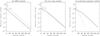 |
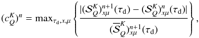
Fig. 3 Maximum relative change of the Stokes I source vector component
|
 (38)with n the
iteration index, τd a depth-grid point, and
(38)with n the
iteration index, τd a depth-grid point, and ![Mathematical equation: \begin{equation} (\overline{{\mathcal S}}^K_Q)^{n+1}_{x\mu}(\tau_{\rm d}) = {1\over 2} \left[ |({{\mathcal S}}^K_Q)^{n+1}_{x\mu}(\tau_{\rm d})| + |({{\mathcal S}}^K_Q)^{n+1}_{x\mu}(\tau_{d+1})|\right]. \label{mrc_denom} \end{equation}](/articles/aa/full_html/2011/03/aa15813-10/aa15813-10-eq242.png) (39)The
(39)The
 yield the maximum
relative change from one iteration to the next for each component
yield the maximum
relative change from one iteration to the next for each component
 . We also
introduce
. We also
introduce  (40)where
P = Q/I is the degree of linear
polarization at the surface. The quantity
(40)where
P = Q/I is the degree of linear
polarization at the surface. The quantity  measures the
progress of iteration on the surface polarization of the radiation field. For the ALI type
methods, the convergence is tested using the criterion
measures the
progress of iteration on the surface polarization of the radiation field. For the ALI type
methods, the convergence is tested using the criterion ![Mathematical equation: \begin{equation} c^n={\rm max} \left[ (c^0_0)^n, c^n_{\rm p} \right] < 10^{-8}. \label{criteria} \end{equation}](/articles/aa/full_html/2011/03/aa15813-10/aa15813-10-eq247.png) (41)In the asymptotic
regime of large n, the components are slave modes of
the component
(41)In the asymptotic
regime of large n, the components are slave modes of
the component  , so all the
have more or less
the same behavior as
, so all the
have more or less
the same behavior as  (see Nagendra et al. 1998). For the scattering expansion
method, we perform two iteration tests, a first one on
when calculating the
component with an ALI method
(first stage), and then a second one on , when
calculating the components
(see Nagendra et al. 1998). For the scattering expansion
method, we perform two iteration tests, a first one on
when calculating the
component with an ALI method
(first stage), and then a second one on , when
calculating the components  (second stage)
with the iteration formula given in Eq. (36). The iterations are stopped when and
become smaller than
10-8.
(second stage)
with the iteration formula given in Eq. (36). The iterations are stopped when and
become smaller than
10-8.
Figure 3 shows the variations in
and
versus the iteration
number. The model parameters used are
(T,a,ϵ,r,ΓE/ΓR) = (2 × 104,10-3,10-4,0,0).
The panel (a) corresponds to the FABFA method, and the panel (b) to the core-wing method.
The convergence behavior of these two new ALI methods is nearly similar to the standard
Polarized ALI (PALI) methods (Nagendra et al. 1999).
The approximation introduced for the core-wing method (see Eq. (22)) does not seem to affect the speed of
convergence significantly. We also find that the speeds of convergence are about the same
for angle-averaged and angle-dependent PRD. The main parameters that can affect the speed of
convergence are the optical thickness of the line (there being faster convergence for
optically thin than optically thick lines), and the frequency grid, coarser grids leading to
faster convergence (Olson et al. 1986). The panel (c)
of Fig. 3 shows the variation in
and
for the scattering
expansion method. The number of iterations in the second iteration stage is clearly small
(~60) compared to the first iteration stage (~140).
To illustrate the convergence properties of the ALI methods, we show in Fig. 4 the convergence history of the four components of
at x = 0 calculated with the core-wing method. To reduce the number of
lines, every fourth iteration solutions are plotted. We note that
 for
x = 0 satisfies the
for
x = 0 satisfies the  law at the surface. As the slab is not optically very thick
(T = 2 × 10⁴), has not fully
reached unity at the mid-slab. All the other components
law at the surface. As the slab is not optically very thick
(T = 2 × 10⁴), has not fully
reached unity at the mid-slab. All the other components
 go to zero at the
mid slab. In the wing frequencies, say x = 4, the rate of convergence for
all the four components of
is quite large (figure not shown here).
go to zero at the
mid slab. In the wing frequencies, say x = 4, the rate of convergence for
all the four components of
is quite large (figure not shown here).
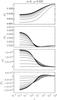 |
Fig. 4 Convergence history of the four components of the
source vector |
Figure 5 shows the convergence history of the
components for
x = 0 and μ = 0.025 calculated with the scattering
expansion method, for the same atmospheric model as in Figs. 3 and 4. The dotted lines indicate the single
scattered solution. For  and
and
 , the single
scattered solution is very close to the converged solution, while for
, the single
scattered solution is very close to the converged solution, while for
 a few iterations
are needed to reach the converged solution. In the last panel of Fig. 5, we show the convergence history for the ratio
Q/I. We have not performed a systematic investigation
of the variation in the speed of convergence with the slab thickness as was done for CRD in
Frisch et al. (2009), but the calculations that we
have performed suggest that the behavior observed with CRD will also hold for
angle-dependent and angle-averaged PRD, namely, a very good approximation to the emergent
polarization is provided by the single scattered solution for optically thin slabs
(T ≪ 10) and optically very thick ones
(T ≥ 2 × 10⁶), but is not reliable for intermediate optical
thicknesses. As shown here, the problem can be cured by considering higher order terms in
the scattering expansion. For example, for a very strong line such as Ca i 4227 Å
the Q/I profile can be fitted fairly well with a single
scattered solution (Anusha et al. 2010), although the
line core is somewhat underestimated. The fit could probably be improved by considering
higher order terms in the scattering expansion.
a few iterations
are needed to reach the converged solution. In the last panel of Fig. 5, we show the convergence history for the ratio
Q/I. We have not performed a systematic investigation
of the variation in the speed of convergence with the slab thickness as was done for CRD in
Frisch et al. (2009), but the calculations that we
have performed suggest that the behavior observed with CRD will also hold for
angle-dependent and angle-averaged PRD, namely, a very good approximation to the emergent
polarization is provided by the single scattered solution for optically thin slabs
(T ≪ 10) and optically very thick ones
(T ≥ 2 × 10⁶), but is not reliable for intermediate optical
thicknesses. As shown here, the problem can be cured by considering higher order terms in
the scattering expansion. For example, for a very strong line such as Ca i 4227 Å
the Q/I profile can be fitted fairly well with a single
scattered solution (Anusha et al. 2010), although the
line core is somewhat underestimated. The fit could probably be improved by considering
higher order terms in the scattering expansion.
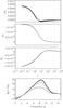 |
Fig. 5 The scattering expansion method. The three
upper panels show the convergence history of the components
|
In terms of computing resources, in particular computing time, the three iterative methods
behave quite differently. In Table 1, we present the
CPU time requirements for the three iterative methods in the case of angle-dependent PRD.
The CPU times spent in specific parts of the computational process are listed, for each of
the methods. The model used is the same as in Figs. 3–5. Since the computation of the azimuthal
Fourier coefficients are
common to all the three iterative methods, they are excluded when estimating the CPU time
requirements. The computing time for can
be huge (several hours) depending on the frequency and angle grids. For each method, the
last but one column in Table 1 gives the number of
iterations multiplied by the CPU time per iteration. This number of iterations is smaller
than the results presented in Fig. 3 because we have
applied the Ng acceleration to all the three iterative methods.
CPU time requirements for the iterative methods after the calculation of the
azimuthal coefficients  ,
Q = 0,1,2.
,
Q = 0,1,2.
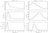 |
Fig. 6 A comparison of emergent Stokes profiles at μ = 0.11 for angle-dependent (solid lines) and angle-averaged (dashed lines) PRD functions. Left panel: slab model with parameters (T,a,ϵ,r,ΓE/ΓR) = (10,10-3,10-4,0,1). Right panel: slab model with parameters (T,a,ϵ,r,ΓE/ΓR) = (2 × 104,10-3,10-4,0,0). |
The scattering expansion method requires the construction of a scalar
Λ∗ operator needed to calculate
in the first stage of
the method. The computation of Λ∗,
, and the single
scattered solution ![Mathematical equation: \hbox{$[\tilde{\mathcal I}_Q^2]^{(1)}$}](/articles/aa/full_html/2011/03/aa15813-10/aa15813-10-eq276.png) requires roughly 3/20th of the total computing time. Thus, most of the time is spent in
calculating the higher order terms in the scattering expansion. For the core-wing method,
almost the entire CPU time is spent in the iterative cycle itself. Each iterative cycle is
about 20% shorter than the time per iteration of the scattering expansion method. In
addition, a larger number of iterations are needed for convergence. It is the need to invert
the large matrix A-1 (see Eq. (19)) that considerably slows down the FABFA
method. We also note that the time per iteration is about three times as long as with the
core-wing method. The CPU times given in Table 1
correspond to the pure RII case
(ΓE/ΓR = 0). The inclusion of collisions does not change the CPU
times for different stages of computational process. The only difference occurs in the
number of iterations required for convergence. The larger the value of
ΓE/ΓR, the smaller the total number of iterations.
requires roughly 3/20th of the total computing time. Thus, most of the time is spent in
calculating the higher order terms in the scattering expansion. For the core-wing method,
almost the entire CPU time is spent in the iterative cycle itself. Each iterative cycle is
about 20% shorter than the time per iteration of the scattering expansion method. In
addition, a larger number of iterations are needed for convergence. It is the need to invert
the large matrix A-1 (see Eq. (19)) that considerably slows down the FABFA
method. We also note that the time per iteration is about three times as long as with the
core-wing method. The CPU times given in Table 1
correspond to the pure RII case
(ΓE/ΓR = 0). The inclusion of collisions does not change the CPU
times for different stages of computational process. The only difference occurs in the
number of iterations required for convergence. The larger the value of
ΓE/ΓR, the smaller the total number of iterations.
For the core-wing and the scattering expansion methods, the computing time per iteration scales as Nd(Nx2Nμ), where Nd is the total number of depth points. For the FABFA method, the total computing time scales as Nd(Nx2Nμ)2. For the FABFA and core-wing methods, the number of iterations can be reduced by using a Gauss-Seidel decomposition or SOR method instead of a Jacobi decomposition. In any case, the FABFA method will remain slow, by a large factor, compared to the core-wing method. We recall that for the perturbation method used in Nagendra et al. (2002), the computing time per iteration scales as Nd(Nx2NμNϕ), with Nϕ the number of azimuths needed to describe the azimuthal variation of the Stokes source vector. The number of iterations required for convergence is around 20.
6. Stokes profiles calculated with angle-dependent and angle-averaged PRD functions
We compare the Stokes parameters I, Q, and the ratio
Q/I calculated with angle-averaged and angle-dependent
PRD functions, for several atmospheric models. The Stokes parameters calculated with
angle-dependent PRD functions are shown as solid lines and those calculated with
angle-averaged PRD functions as dashed lines. The results are analyzed with the help of the
decomposition, which
may be written as  (42)We
recall that the irreducible components depend on
τ, x, and μ. The contributions of the
component
(42)We
recall that the irreducible components depend on
τ, x, and μ. The contributions of the
component  go to zero at both
the limb and the disk center, for both Stokes I and Stokes
Q.
go to zero at both
the limb and the disk center, for both Stokes I and Stokes
Q.
In Fig. 6, we show the emergent I,
Q/I, and Q profiles at
μ = 0.11 for angle-dependent and angle-averaged PRD functions. The
angle-averaged solution is calculated with the PALI method of Fluri et al. (2003) and the angle-dependent solution with the core-wing
method introduced here. In the left-hand side panels, T = 10 and the PRD
used is an equal mixture of rII and
rIII. In the right-hand side panels,
T = 2 × 10⁴ and the PRD used is pure
rII. Figure 6 clearly
shows that the angle-averaged and angle-dependent solutions may differ significantly and
that the angle-averaged emergent polarization may be smaller or larger than the
angle-dependent one. We now try to explain the reasons for this, by considering the
components .
In Fig. 7, we show the components
corresponding to the
two atmospheric models in Fig. 6. The components with
Q ≠ 0 are zero for the angle-averaged PRD functions. The components
are essentially equal
for the AD and AA cases when T = 10, while they slightly differ around
x = 3 when T = 2 × 10⁴. Since Stokes
I is dominated by , it is also
nearly independent of the choice of the PRD function. Stokes Q consists of
the three components  ,
, and
,
, and
 . We can observe that
has very different
values in the AD and AA cases, being smaller in absolute value in the AD case. This is a
somewhat unexpected result. The reason for the difference between the AA and AD results is
the use of
. We can observe that
has very different
values in the AD and AA cases, being smaller in absolute value in the AD case. This is a
somewhat unexpected result. The reason for the difference between the AA and AD results is
the use of  in the AD
case and the angle-averaged redistribution function
in the AD
case and the angle-averaged redistribution function  in the AA
case.
in the AA
case.
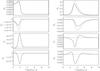 |
Fig. 7 A comparison of emergent
|
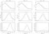 |
Fig. 8 Stokes I and Q/I profiles at the surface for different values of the heliocentric angle computed for the angle-averaged (dashed lines) and the angle-dependent (solid lines) PRD. The bottom three panels show the absolute difference in Q/I between the AA and AD profiles. The atmospheric model used is (T,a,ϵ,r,ΓE/ΓR) = (2 × 104,10-3,10-4,0,0). |
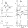 |
Fig. 9 The μ dependence of the irreducible
components of ℐ (left panels) and
|
Equation (42) shows that for small values
of μ, only and
contribute to Stokes
Q and that  . For T = 10, the
two terms have the same sign and when added together give a value of Stokes
Q that is slightly smaller in the AD case than in the AA case. For
spectral lines with a small optical thickness, the role of PRD is essentially negligible.
These lines can be modeled reasonably well with CRD (Sampoorna et al. 2010). Thus, one may not expect large differences between
angle-averaged and angle-dependent polarization profiles. For
T = 2 × 10⁴, and
are mainly negative,
with having a slightly
larger absolute value than . When added
together, they give a negative value, but because of the minus sign, one ends up with a
positive Stokes Q, which is however smaller than the corresponding AA
Stokes Q.
. For T = 10, the
two terms have the same sign and when added together give a value of Stokes
Q that is slightly smaller in the AD case than in the AA case. For
spectral lines with a small optical thickness, the role of PRD is essentially negligible.
These lines can be modeled reasonably well with CRD (Sampoorna et al. 2010). Thus, one may not expect large differences between
angle-averaged and angle-dependent polarization profiles. For
T = 2 × 10⁴, and
are mainly negative,
with having a slightly
larger absolute value than . When added
together, they give a negative value, but because of the minus sign, one ends up with a
positive Stokes Q, which is however smaller than the corresponding AA
Stokes Q.
We now examine how the differences between the AD and AA polarizations vary with the position on the disk, the optical thickness T of the slab, the thermalization parameter ϵ, the value of the continuum absorption, and the ratio ΓE/ΓR.
6.1. Center-to-limb variations
We know that the angle-dependent PRD functions become azimuthally symmetric at the disk center. Thus we can expect the AD and AA polarization profiles to become very close to each other when μ → 1. This is indeed what we observe in Fig. 8 where we show the emergent profiles of Stokes I and the ratio Q/I. In the bottom three panels, we show the absolute difference between the AA and AD Q/I profiles. As μ → 1, the absolute difference clearly goes to zero.
We show in Fig. 9 the dependence on
μ of the components and
 at the
surface. For , the
dependence on μ comes from the AD redistribution functions
at the
surface. For , the
dependence on μ comes from the AD redistribution functions
 (see Eq. (13)). We recall that the source vector
components are independent of μ for AA-PRD. For the components
, the variations
with μ are caused by the limb-darkening and the
μ-variation in the source vector components. In the right panels of
Fig. 9, we can observe that
is almost
independent of μ and we can verify that
,
Q = 1,2, go to zero when μ is close to one. The
variation in is rather
monotonic, but that of is not. The
component increases
towards the disk center, as it is controlled by the magnitude of
(see Eq. (13)). We recall that the source vector
components are independent of μ for AA-PRD. For the components
, the variations
with μ are caused by the limb-darkening and the
μ-variation in the source vector components. In the right panels of
Fig. 9, we can observe that
is almost
independent of μ and we can verify that
,
Q = 1,2, go to zero when μ is close to one. The
variation in is rather
monotonic, but that of is not. The
component increases
towards the disk center, as it is controlled by the magnitude of
 (see dotted
lines in panel of
Fig. 5). In the left panels of Fig. 9, one can verify that
increases
from the limb to the disk center, while the components
,
Q = 1,2, go to zero at the disk center.
(see dotted
lines in panel of
Fig. 5). In the left panels of Fig. 9, one can verify that
increases
from the limb to the disk center, while the components
,
Q = 1,2, go to zero at the disk center.
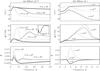 |
Fig. 10 The emergent I, Q/I, and Q profiles at μ = 0.11 computed for the angle-averaged (dashed lines) and the angle-dependent (solid lines) PRD. Left panel shows the effect of optical thickness T when ϵ = 10-4. Different line types are: thin lines T = 2 × 10⁴, medium thick lines T = 2 × 10⁶, and thick lines T = 2 × 10⁸. Inset in Q/I panel shows T = 2 × 10⁸ case for a larger frequency range. Right panel shows the effect of ϵ for optical thickness T = 2 × 10⁴. Different line types are: thin lines ϵ = 10-2, medium thick lines ϵ = 10-6, and thick lines ϵ = 0. Remaining common parameters are (a,r,ΓE/ΓR) = (10-3,0,0). |
6.2. Effects of the optical thickness T and thermalization parameter ϵ
In Fig. 10, we compare the angle-averaged and the corresponding angle-dependent Stokes I, Q, and Q/I profiles for slabs with different values of the optical thickness T and the thermalization parameter ϵ. For the angle-dependent case, the calculations were performed with the core-wing method. For all the examples shown in Fig. 10, the optical thickness is equal to or larger than 2 × 10⁴. One can observe that the ratio Q/I is always smaller for the angle-dependent than for the angle-averaged PRD functions. This situation appears to be typical of optically thick lines in isothermal atmospheres (see also Nagendra et al. 2002).
In the left panels, ϵ = 10-4. The three values chosen for T correspond to effectively thin (ϵT = 2), effectively thick (ϵT = 200), and semi-infinite like conditions (ϵT = 2 × 10⁴). The amplitudes of Q/I and Q in the near wing peaks decrease with increasing T. For Q/I, this is accompanied by a decrease in the differences between the angle-averaged and angle-dependent values. In the particular case of T = 2 × 10⁸, typical features of semi-infinite atmospheres can be observed. For example, the appearance of double peaks – one narrow peak in the near wings, and a second broader one in the far wings – is a typical behavior of Q/I in strong resonance lines such as that of the Ca ii K line (see e.g., Stenflo 1980; Holzreuter et al. 2006).
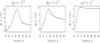 |
Fig. 11 The emergent Q/I profiles at μ = 0.11 computed for the angle-averaged (dashed lines) and the angle-dependent (solid lines) PRD. The model parameters are (T,a,ϵ,ΓE/ΓR) = (2 × 104,10-3,10-4,0). The parameter r takes the values 10-8, 10-6, and 10-4. |
In the right panels of Fig. 10, the optical thickness is T = 2 × 10⁴. As ϵ increases from 10-6 (effectively thin, ϵT = 2 × 10⁻²) to 10-2 (effectively thick, ϵT = 2 × 10²), the magnitudes of both I and Q increase because the number of photons that are emitted increases, as does the strength of the coupling between the radiation field and the thermal pool. However, the ratio Q/I decreases because the number of polarized photons is reduced by the thermalization of the radiation field (see e.g., Saliba 1986). For ϵ = 10-6, the angle-averaged and angle-dependent profiles display significant differences in the Q/I profiles. This difference decreases when ϵ = 10-2.
We also considered the case ϵ = 0 (conservative scattering). In this case, there are no internal sources of photons (ϵB = 0), but there is an incident field at the lower boundary I(τ = T,x,μ) = B. For this model, the primary source of photons G0(τ) decreases towards the surface at τ = 0. For the emergent Stokes I and Q profiles, the differences between the angle-averaged and angle-dependent cases are insignificant. Some differences appear however in the ratio Q/I around the line center (0 < x < 4).
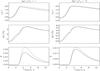 |
Fig. 12 The emergent Stokes parameters I and Q and the ratio Q/I at μ = 0.11 computed for the angle-averaged (dashed lines) and the angle-dependent (solid lines) PRD. The model parameters are (T,a,ϵ,r) = (2 × 104,10-3,10-4,0). The parameter ΓE/ΓR takes the values 1 and 10. |
6.3. Effect of the continuum strength parameter r
All the results shown in the previous figures were obtained with a continuum absorption set to zero. In Fig. 11, we show the Q/I profile for values of the continuum strength parameter r set to 10-8, 10-6, and 10-4. The atmospheric model is the same as in Fig. 6b except for the value of r. When r increases, one can observe a significant decrease in amplitude of the near wing peak, an effect already investigated in Faurobert (1988), and a gradual disappearance of the differences between the angle-averaged and angle-dependent Q/I profiles. For r = 10-2 (result not shown here), the differences become essentially zero.
6.4. Effect of the elastic collisions ΓE
A change in the value of ΓE, modifies the coherency factor γcoh defined in Sect. 5, hence the relative contributions of rII and rIII. It is well established that the wings of Stokes I and the linear polarization are quite sensitive to the PRD mechanism (Nagendra et al. 2002). We show in Fig. 12 the Stokes parameters I and Q, and the ratio Q/I calculated with the angle-averaged and angle-dependent PRD functions with the core-wing method. We show two examples, ΓE/ΓR = 1, which corresponds to an even mixture of rII and rIII, and ΓE/ΓR = 10, which corresponds to an uneven mixture of rII and rIII with a dominant contribution from rIII. For D(2), we assume the relation D(2) = 0.5ΓE. We can observe that the polarization rate decreases as ΓE/ΓR increases, a phenomenon discussed in detail in Nagendra et al. (2002). The differences between the AA and AD Stokes I and Q profiles decrease as ΓE/ΓR increases. For ΓE/ΓR > 100, these differences become insignificant.
7. Conclusions
We have investigated the Rayleigh scattering with angle-dependent partial redistribution (PRD) functions to evaluate the reliability of the usual angle-averaged approximation. The analysis has been carried out for a two-level atom with unpolarized ground level using the angle-dependent PRD functions established in Domke & Hubeny (1988); Bommier (1997a). The scattering medium has been assumed to be a plane-parallel, cylindrically symmetrical, isothermal slab. For this model, the polarized radiation field is cylindrically symmetrical (i.e. depends only on the inclination θ with respect to the direction perpendicular to the slab surface) and can be represented by the two Stokes parameters I and Q. The source terms in the transfer equations for I and Q have a complicated dependence on the angle θ, because it appears in the polarization phase matrix and also in the angle-dependent PRD functions. It was shown in HF10 that the polarized radiation field can be decomposed into four components that are cylindrically symmetrical and satisfy standard radiative transfer equations. The source terms still depend on θ but in a much simpler way. Thanks to this decomposition method, we have been able to construct three different iterative methods of solution for the calculation of the Stokes parameters. Two are of the accelerated lambda iteration (ALI) type; they are generalizations of the frequency-by-frequency (FBF) and core-wing methods originally formulated for scalar PRD transfer in Paletou & Auer (1995). The other is a scattering expansion (Neumann series) method developed for the Hanle effect with complete frequency redistribution in Frisch et al. (2009).
Crucial ingredients for the three methods are the azimuthal Fourier coefficients of order 0,1, and 2 of the angle-dependent Hummer’s (1962) PRD functions rII and rIII. The calculations of these Fourier coefficients is quite time consuming, in particular for rIII, because very fine grids are needed to properly represent their sharp variations with the frequency and inclination of the incident and scattered beams. Once these coefficients have been calculated, and also an approximate solution of Stokes I (neglecting polarization) is obtained in the scattering expansion method, the core-wing and scattering expansion approaches both provide fast and accurate solutions. The scattering expansion method appears particularly interesting in problems of large dimensionality (very large number of frequency, angle, and depth grid points).
We have found that the angle-averaged PRD functions overestimate the emergent polarization rate Q/I between 10% and 30% for slabs with a large optical thickness (between 2 × 10⁴ and 2 × 10⁸), the largest differences occurring in the near wing peaks. For optically thin slabs, the differences are much smaller. We have not considered semi-infinite atmospheres. As the difference between the polarization rates obtained with angle-averaged and angle-dependent PRD functions remain fairly small, the sign of this difference may easily depend on the particular choice of the atomic and atmospheric model. It would certainly be interesting to consider realistic solar atmosphere models as has recently been done in Sampoorna et al. (2010). The numerical methods we have proposed here are able to do this. This type of analysis would certainly help us to understand the discrepancies between observed polarization rates and theoretical predictions (Anusha et al. 2010).
For the weak-field Hanle effect, the reliability of the angle-averaged approximation for PRD functions is clearly questionable, for Stokes Q and especially Stokes U (Nagendra et al. 2002). In the presence of a weak magnetic field, the polarized radiation field can be decomposed into a set of six irreducible components. For an angle-dependent PRD, these components have no cylindrical symmetry, but a Fourier azimuthal expansion allows one to construct an infinite set of integral equations similar to the equations given here (Frisch 2009). The core-wing or a scattering expansion method applied to a truncated set of these equations offer some hope in calculating the polarization with a reasonable amount of numerical work.
We recall that for these three different types of redistribution functions the lower level is infinitely sharp; for type I, the upper level is also sharp, for type II, the upper level is radiatively broadened, and for type III, it is also broadened by collisions.
Although the redistribution functions are not even functions of , because the radiation field is an even function of , only positive values of can be considered.
Acknowledgments
The authors are grateful to Dr. V. Bommier for providing a FORTRAN PROGRAM to compute angle-dependent type III redistribution function and to L. S. Anusha for helpful discussions.
References
- Adams, T. F., Hummer, D. G., & Rybicki, G. B. 1971, ApJ, 11, 1365 [Google Scholar]
- Anusha, L. S., Nagendra, K. N., Stenflo, J. O., et al. 2010, ApJ, 718, 988 [NASA ADS] [CrossRef] [Google Scholar]
- Bommier, V. 1997a, A&A, 328, 706 [NASA ADS] [Google Scholar]
- Bommier, V. 1997b, A&A, 328, 726 [NASA ADS] [Google Scholar]
- Chandrasekhar, S. 1950, Radiative transfer (Oxford: Clarendon Press) [Google Scholar]
- Domke, H., & Hubeny, I. 1988, ApJ, 334, 527 [NASA ADS] [CrossRef] [Google Scholar]
- Dumont, S., Omont, A., Pecker, J. C., & Rees, D. E. 1977, A&A, 54, 675 [NASA ADS] [Google Scholar]
- Faurobert, M. 1987, A&A, 178, 269 [NASA ADS] [Google Scholar]
- Faurobert, M. 1988, A&A, 194, 268 [NASA ADS] [Google Scholar]
- Faurobert-Scholl, M. 1991, A&A, 246, 469 [NASA ADS] [Google Scholar]
- Fluri, D. M., Nagendra, K. N., & Frisch, H. 2003, A&A, 400, 303 [NASA ADS] [CrossRef] [EDP Sciences] [Google Scholar]
- Frisch, H. 2007, A&A, 476, 665 [NASA ADS] [CrossRef] [EDP Sciences] [Google Scholar]
- Frisch, H. 2009, in Solar Polarization 5, ed. S. V. Berdyugina, K. N. Nagendra, & R. Ramelli (San Francisco: ASP), ASP Conf. Ser., 405, 87 [Google Scholar]
- Frisch, H. 2010, A&A, 522, A41 (HF10) [NASA ADS] [CrossRef] [EDP Sciences] [Google Scholar]
- Frisch, H., Anusha, L. S., Sampoorna, M., & Nagendra, K. N. 2009, A&A, 501, 335 [NASA ADS] [CrossRef] [EDP Sciences] [Google Scholar]
- Holzreuter, R., Fluri, D. M., & Stenflo, J. O. 2006, A&A, 449, L41 [NASA ADS] [CrossRef] [EDP Sciences] [Google Scholar]
- Hummer, D. G. 1962, MNRAS, 125, 21 [NASA ADS] [CrossRef] [Google Scholar]
- Landi Degl’Innocenti, E. 1984, Sol. Phys., 91, 1 [NASA ADS] [CrossRef] [Google Scholar]
- Landi Degl’Innocenti, E., & Landolfi, M. 2004, Polarization in Spectral Lines (Dordrecht: Kluwer) [Google Scholar]
- Manso Sainz, R., & Trujillo Bueno, J. 1999, in Solar Polarization, ed. K. N. Nagendra, & J. O. Stenflo (Boston: Kluwer), 143 [Google Scholar]
- McKenna, S. J. 1985, Ap&SS, 108, 31 [NASA ADS] [CrossRef] [Google Scholar]
- Milkey, R. W., Shine, R. A., & Mihalas, D. 1975, ApJ, 202, 250 [NASA ADS] [CrossRef] [Google Scholar]
- Nagendra, K. N. 1988, ApJ, 335, 269 [NASA ADS] [CrossRef] [Google Scholar]
- Nagendra, K. N. 1994, ApJ, 432, 274 [NASA ADS] [CrossRef] [Google Scholar]
- Nagendra, K. N. 2003, in Stellar atmosphere modeling, ed. I. Hubeny, D. Mihalas, & K. Werner (San Francisco: ASP), ASP Conf. Ser., 288, 583 [Google Scholar]
- Nagendra, K. N., & Sampoorna, M. 2009, in Solar Polarization 5, ed. S. V. Berdyugina, K. N. Nagendra, & R. Ramelli (San Francisco: ASP), ASP Conf. Ser., 405, 261 [Google Scholar]
- Nagendra, K. N., Frisch, H., & Faurobert-Scholl, M. 1998, A&A, 332, 610 [NASA ADS] [Google Scholar]
- Nagendra, K. N., Paletou, F., Frisch, H., & Faurobert-Scholl, M. 1999, in Solar Polarization, ed. K. N. Nagendra, & J. O. Stenflo (Boston: Kluwer), 127 [Google Scholar]
- Nagendra, K. N., Frisch, H., & Faurobert, M. 2002, A&A, 395, 305 [NASA ADS] [CrossRef] [EDP Sciences] [Google Scholar]
- Nagendra, K. N., Frisch, H., & Fluri, D. M. 2003, in Solar Polarization, ed. J. Trujillo Bueno, & J. Sanchez Almeida (San Francisco: ASP), ASP Conf. Ser. 307, 227 [Google Scholar]
- Olson, G. L., Auer, L. H., & Buchler, J. R. 1986, J. Quant. Spec. Radiat. Transf., 35, 431 [NASA ADS] [CrossRef] [Google Scholar]
- Paletou, F., & Auer, L. H. 1995, A&A, 297, 771 [NASA ADS] [Google Scholar]
- Rees, D. E., & Saliba, G. J. 1982, A&A, 115, 1 [NASA ADS] [Google Scholar]
- Saliba, G. J. 1986, Ph.D. Thesis, Univ. of Sidney [Google Scholar]
- Sampoorna, M., & Trujillo Bueno, J. 2010, ApJ, 712, 1331 [NASA ADS] [CrossRef] [Google Scholar]
- Sampoorna, M., Nagendra, K. N., & Stenflo, J. O. 2007a, ApJ, 663, 625 [NASA ADS] [CrossRef] [Google Scholar]
- Sampoorna, M., Nagendra, K. N., & Stenflo, J. O. 2007b, ApJ, 670, 1485 [NASA ADS] [CrossRef] [Google Scholar]
- Sampoorna, M., Nagendra, K. N., & Stenflo, J. O. 2008a, ApJ, 679, 889 [NASA ADS] [CrossRef] [Google Scholar]
- Sampoorna, M., Nagendra, K. N., & Frisch, H. 2008b, J. Quant. Spec. Radiat. Transf., 109, 2349 [Google Scholar]
- Sampoorna, M., Trujillo Bueno, J., & Landi Degl’Innocenti, E. 2010, ApJ, 722, 1269 [NASA ADS] [CrossRef] [Google Scholar]
- Stenflo, J. O. 1980, A&A, 84, 68 [NASA ADS] [Google Scholar]
- Trujillo Bueno, J., & Fabiani Bendicho, P. 1995, ApJ, 455, 646 [NASA ADS] [CrossRef] [Google Scholar]
- Trujillo Bueno, J., & Manso Sainz, R. 1999, ApJ, 516, 436 [NASA ADS] [CrossRef] [Google Scholar]
- Vardavas, I. M. 1976, J. Quant. Spec. Radiat. Transf., 16, 1 [NASA ADS] [CrossRef] [Google Scholar]
- Wallace, L., & Yelle, R. V. 1989, ApJ, 346, 489 [NASA ADS] [CrossRef] [Google Scholar]
All Tables
CPU time requirements for the iterative methods after the calculation of the
azimuthal coefficients ,
Q = 0,1,2.
All Figures
|
Fig. 1 Surface plots of azimuth averaged redistribution functions of type II (left panels) and of type III (right panels) with Q = 0. The X-axis represents the outgoing frequency x, and the Y-axis represents outgoing direction μ. The incoming direction is μ′ = 0.3. The damping parameter a = 0.001. The top two panels correspond to the incoming frequency x′ = 3, and the bottom panels to x′ = 4. |
| In the text | |
|
Fig. 2 Azimuth averaged redistribution functions of type II (left panels) and of type III (right panels), plotted as a function of the outgoing frequency x, for different choices of μ, and μ′. The damping parameter a = 0.001. Thin lines correspond to x′ = 1 and thick lines to x′ = 4. Solid, dotted and dashed lines correspond respectively to Q = 0,1, and 2. |
| In the text | |
|
Fig. 3 Maximum relative change of the Stokes I source vector component
|
| In the text | |
|
Fig. 4 Convergence history of the four components of the
source vector |
| In the text | |
|
Fig. 5 The scattering expansion method. The three
upper panels show the convergence history of the components
|
| In the text | |
|
Fig. 6 A comparison of emergent Stokes profiles at μ = 0.11 for angle-dependent (solid lines) and angle-averaged (dashed lines) PRD functions. Left panel: slab model with parameters (T,a,ϵ,r,ΓE/ΓR) = (10,10-3,10-4,0,1). Right panel: slab model with parameters (T,a,ϵ,r,ΓE/ΓR) = (2 × 104,10-3,10-4,0,0). |
| In the text | |
|
Fig. 7 A comparison of emergent
|
| In the text | |
|
Fig. 8 Stokes I and Q/I profiles at the surface for different values of the heliocentric angle computed for the angle-averaged (dashed lines) and the angle-dependent (solid lines) PRD. The bottom three panels show the absolute difference in Q/I between the AA and AD profiles. The atmospheric model used is (T,a,ϵ,r,ΓE/ΓR) = (2 × 104,10-3,10-4,0,0). |
| In the text | |
|
Fig. 9 The μ dependence of the irreducible
components of ℐ (left panels) and
|
| In the text | |
|
Fig. 10 The emergent I, Q/I, and Q profiles at μ = 0.11 computed for the angle-averaged (dashed lines) and the angle-dependent (solid lines) PRD. Left panel shows the effect of optical thickness T when ϵ = 10-4. Different line types are: thin lines T = 2 × 10⁴, medium thick lines T = 2 × 10⁶, and thick lines T = 2 × 10⁸. Inset in Q/I panel shows T = 2 × 10⁸ case for a larger frequency range. Right panel shows the effect of ϵ for optical thickness T = 2 × 10⁴. Different line types are: thin lines ϵ = 10-2, medium thick lines ϵ = 10-6, and thick lines ϵ = 0. Remaining common parameters are (a,r,ΓE/ΓR) = (10-3,0,0). |
| In the text | |
|
Fig. 11 The emergent Q/I profiles at μ = 0.11 computed for the angle-averaged (dashed lines) and the angle-dependent (solid lines) PRD. The model parameters are (T,a,ϵ,ΓE/ΓR) = (2 × 104,10-3,10-4,0). The parameter r takes the values 10-8, 10-6, and 10-4. |
| In the text | |
|
Fig. 12 The emergent Stokes parameters I and Q and the ratio Q/I at μ = 0.11 computed for the angle-averaged (dashed lines) and the angle-dependent (solid lines) PRD. The model parameters are (T,a,ϵ,r) = (2 × 104,10-3,10-4,0). The parameter ΓE/ΓR takes the values 1 and 10. |
| In the text | |
Current usage metrics show cumulative count of Article Views (full-text article views including HTML views, PDF and ePub downloads, according to the available data) and Abstracts Views on Vision4Press platform.
Data correspond to usage on the plateform after 2015. The current usage metrics is available 48-96 hours after online publication and is updated daily on week days.
Initial download of the metrics may take a while.