| Issue |
A&A
Volume 525, January 2011
|
|
|---|---|---|
| Article Number | A155 | |
| Number of page(s) | 8 | |
| Section | The Sun | |
| DOI | https://doi.org/10.1051/0004-6361/201015479 | |
| Published online | 10 December 2010 | |
Alfvén wave phase-mixing and damping in the ion cyclotron range of frequencies
1
School of Mathematics and Statistics, University of St.
Andrews,
St. Andrews,
Fife
KY16 9SS,
UK
e-mail: jamest@mcs.st-and.ac.uk; ineke@mcs.st-and.ac.uk
2
EURATOM/CCFE Fusion Association, Culham Science Centre, Abingdon,
Oxfordshire,
OX14 3DB,
UK
e-mail: k.g.mcclements@ccfe.ac.uk
Received:
27
July
2010
Accepted:
18
October
2010
Aims. We determine the effect of the Hall term in the generalised Ohm’s law on the damping and phase mixing of Alfvén waves in the ion cyclotron range of frequencies in uniform and non-uniform equilibrium plasmas.
Methods. Wave damping in a uniform plasma is treated analytically, whilst a Lagrangian remap code (Lare2d) is used to study Hall effects on damping and phase mixing in the presence of an equilibrium density gradient.
Results. The magnetic energy associated with an initially Gaussian field
perturbation in a uniform resistive plasma is shown to decay algebraically at a rate that
is unaffected by the Hall term to leading order in  where k is wavenumber and δi is ion skin
depth. A similar algebraic decay law applies to whistler perturbations in the limit
where k is wavenumber and δi is ion skin
depth. A similar algebraic decay law applies to whistler perturbations in the limit
 . In a
non-uniform plasma it is found that the spatially-integrated damping rate due to phase
mixing is lower in Hall MHD than it is in MHD, but the reduction in the damping rate,
which can be attributed to the effects of wave dispersion, tends to zero in both the weak
and strong phase mixing limits.
. In a
non-uniform plasma it is found that the spatially-integrated damping rate due to phase
mixing is lower in Hall MHD than it is in MHD, but the reduction in the damping rate,
which can be attributed to the effects of wave dispersion, tends to zero in both the weak
and strong phase mixing limits.
Key words: plasmas / waves / magnetohydrodynamics (MHD) / Sun: flares / Sun: chromosphere
© ESO, 2010
1. Introduction
The interaction between Alfvén waves and plasma inhomogeneities forms a well-studied and important area of research, for both laboratory and astrophysical plasmas. One process which arises as a result of this interaction is Alfvén wave phase-mixing. Early studies of Alfvén wave phase-mixing demonstrated a potential for significantly enhanced plasma heating. In particular, Heyvaerts & Priest (1983) proposed the phase-mixing of Alfvén waves as a potential solar coronal heating mechanism through enhanced wave-dissipation. They outlined that for a magnetohydrodynamic (MHD) treatment of initially planar shear-Alfvén waves, propagating independently on individual magnetic surfaces, large differences in phase are quickly generated between waves on neighbouring field lines, as a result of variation in Alfvén speed across the field. These phase-differences generate progressively smaller scales, and dramatically enhance the effects of viscous and Ohmic dissipation, in the locations where the Alfvén speed gradient is steepest.
This initial concept has been subsequently adapted for a variety of problems using MHD, based on the premise that the waves in question arise as a result of an infinite series of boundary motions at the photosphere. For example, this treatment has been used to investigate the heating of open magnetic field lines under various conditions, e.g. by Parker (1991); Hood et al. (1997); De Moortel et al. (1999, 2000). Phase-mixing has also been studied as a source of non-linear coupling to other wave modes (see, e.g. Nakariakov et al. 1997; Botha et al. 2000).
Of particular interest for this paper is the work of Hood et al. (2002). They note that an infinite series of boundary motions is unrealistic and instead investigate the effect on the amplitude damping rate due to phase-mixing when the waves are driven by only one or two initial impulsive motions at the boundary.
Recent studies have also begun to move away from the original MHD treatment, instead focussing on full kinetic descriptions of a plasma undergoing phase-mixing in a collisionless regime, as a potential mechanism for electron acceleration (see, e.g. Génot et al. 2004; Tsiklauri et al. 2005; Tsiklauri & Haruki 2008; Bian & Kontar 2010). On the assumption that the wavelengths of interest (λ) are small compared to the particle mean free path λmfp, Tsiklauri et al. (2005) and Bian & Kontar (2010) model the corona as a collisionless plasma and cite Landau damping as their primary wave dissipation mechanism. Such damping is strongly suppressed if λ ≫ λmfp (Ono & Kulsrud 1975), as in the case of propagating EUV disturbances with periods of tens or hundreds of seconds (see e.g. De Moortel 2009, and references therein), and a fluid model is then appropriate for the coronal plasma. On the other hand for waves with frequencies approaching the ion cyclotron frequency, typical coronal parameters correspond to classical (Spitzer) collisional mean free paths that exceed λ, suggesting instead the validity of the collisionless approach. However, Craig & Litvinenko (2002) have shown that it is not appropriate to use classical resistivity under flaring conditions because it implies current scale lengths that are several orders of magnitude shorter than λmfp, and moreover is inconsistent with the electric fields required to account for the observed acceleration of protons to tens of MeV on timescales of the order of one second (Hamilton et al. 2003). Craig & Litvinenko proposed that the effective resistivity under flaring conditions (specifically in a reconnecting current sheet) is determined by turbulence arising from electron-ion drift (e.g. ion acoustic) instabilities, and deduced that this effective resistivity could exceed the classical value by a factor of around 106. Under these circumstances a fluid model can be appropriate even for relatively high frequency waves. This may also be true in the upper chromosphere, where the plasma is both cooler and denser (and consequently much more collisional) than in the corona.
It is well known that the electron inertia term in the generalised Ohm’s law becomes comparable to the MHD terms when the system lengthscale approaches the electron skin depth, δe, which in a low beta plasma can exceed the ion Larmor radius. Moreover for perturbations with frequencies approaching the ion cyclotron frequency Ωi, the Hall term in the generalised Ohm’s law becomes as important as the MHD terms when the lengthscale of the system approaches the ion skin depth δi ( ≫ δe). When the introduction of the Hall term into Ohm’s law is the only modification made to the otherwise standard set of MHD equations, we may refer to this as a Hall MHD system.
Hall MHD has been found to be important for a number of fundamental plasma processes. For example, in magnetic reconnection studies, Birn et al. (2001) found that all models which included Hall dynamics returned indistinguishable reconnection rates, concluding that the inclusion of the Hall term is the minimum requirement for fast reconnection (for a summary of Geospace Environmental Modelling (GEM) challenge results, see Birn & Priest 2007).
High frequency waves (i.e. with frequencies ω ~ Ωi), have been observed in a range of astrophysical plasma systems, for example in the solar corona (summarised in Marsch 2006) and in situ, at the Earth’s bow shock (Sckopke et al. 1990). When oscillations in this frequency range are excited in collision-dominated plasmas, such that the collisional mean free path is less than the wavelength, it is then appropriate to use a Hall MHD model.
The goal of our work is to determine the extent to which the main consequences of phase-mixing (wave dissipation and plasma heating) are affected solely by the addition of the Hall term to Ohm’s law. To do this, we first investigate the damping rate of a uniform plasma using Hall MHD (Sect. 2). Phase-mixing is then included, by allowing the equilibrium density to vary (Sect. 2.3). Numerical simulations of a Hall MHD system, with various density profiles and Hall term strengths, are described in Sect. 3. We interpret these results and present conclusions in Sect. 4.
2. Wave damping analysis
The Hall MHD form of Ohm’s Law is
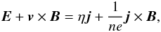 where
E and B are electric and
magnetic fields, v is the single-fluid plasma velocity,
j is current density, η is electrical
resistivity, n is plasma number density and − e is
electron charge. Linearising the induction equation corresponding to this form of Ohm’s law,
together with the equation of motion (neglecting the pressure gradient force), for a plasma
with a uniform equilibrium field
B0 = B0ŷ
for a constant B0, uniform number density and resistivity, and
zero equilibrium flow, gives:
where
E and B are electric and
magnetic fields, v is the single-fluid plasma velocity,
j is current density, η is electrical
resistivity, n is plasma number density and − e is
electron charge. Linearising the induction equation corresponding to this form of Ohm’s law,
together with the equation of motion (neglecting the pressure gradient force), for a plasma
with a uniform equilibrium field
B0 = B0ŷ
for a constant B0, uniform number density and resistivity, and
zero equilibrium flow, gives: ![\begin{eqnarray} \label{eq:HallInduct_L} \frac{\partial{\vec{B}_1}}{\partial t}&\!\!=\!\!&\curl\left({{\vec{v}}\times{\vec{B}_0}}\right)+\frac{\eta}{\muo}\boldnabla^2{\vec{B}_1} \!-\!\frac{1}{\muo ne}\curl\left[\left(\curl{\vec{B}_1}\right)\times{\vec{B}_0} \right] \\ \label{eq:EOM_L} \frac{\partial{\vec{v}}}{\partial{t}}&=&\frac{1}{{\rho_0}\muo}\left(\curl{\vec{B}_1}\right)\times{\vec{B}_0}, \end{eqnarray}](/articles/aa/full_html/2011/01/aa15479-10/aa15479-10-eq23.png) where
B1 [ = (Bx,0,Bz) ]
now represents a transverse perturbation to the equilibrium field,
ρ0 is equilibrium mass density, and
μ0 is the permeability of free space. Note that although, for
simplicity, we neglect plasma pressure, by assuming β = 0 in this
analytical treatment (as Alfvén, whistler and ion cyclotron waves are all incompressible in
a linear regime), the numerical simulations presented in Sect. 3 incorporate plasma pressure, i.e. β ≠ 0.
where
B1 [ = (Bx,0,Bz) ]
now represents a transverse perturbation to the equilibrium field,
ρ0 is equilibrium mass density, and
μ0 is the permeability of free space. Note that although, for
simplicity, we neglect plasma pressure, by assuming β = 0 in this
analytical treatment (as Alfvén, whistler and ion cyclotron waves are all incompressible in
a linear regime), the numerical simulations presented in Sect. 3 incorporate plasma pressure, i.e. β ≠ 0.
By inserting (2) into the time derivative
of (1) in the usual manner, the linearised
Alfvén wave equation is then modified: 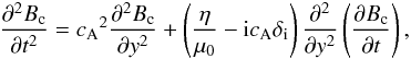 (3)where
we have expressed transverse field perturbations in the form of a complex variable
Bc = Bz + iBx,
and introduced the Alfvén speed,
(3)where
we have expressed transverse field perturbations in the form of a complex variable
Bc = Bz + iBx,
and introduced the Alfvén speed,  ,
and the ion skin depth,
,
and the ion skin depth, 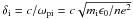 ,
where mi is the ion mass, c is the speed of
light, and ϵ0 is the permittivity of free space.
,
where mi is the ion mass, c is the speed of
light, and ϵ0 is the permittivity of free space.
Seeking wave-like solutions of the form exp(i[ky − ωt])
allows us to form a dispersion relation to express perturbation frequencies,
ω, as a function of wavenumber k. By considering only
the regime of weak damping ( ), we obtain two separate solutions
depending on the size of the parameter
), we obtain two separate solutions
depending on the size of the parameter  . Taking first the
case of
. Taking first the
case of  , we make use of a simple Taylor
expansion to find (to leading order in ):
, we make use of a simple Taylor
expansion to find (to leading order in ): 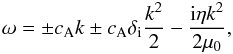 (4)which describes a shear
Alfvén wave, modified by Hall effects, and subject to resistive damping.
(4)which describes a shear
Alfvén wave, modified by Hall effects, and subject to resistive damping.
Considering the opposite case, when  , we find:
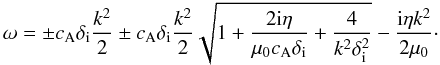 Including the next term in
the Taylor expansion, we find two distinct forward propagating solutions:
Including the next term in
the Taylor expansion, we find two distinct forward propagating solutions: 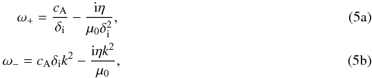 where
in this limit, we now obtain a combination of whistler and ion cyclotron (i.c.) waves, both
subject to a form of resistive damping.
where
in this limit, we now obtain a combination of whistler and ion cyclotron (i.c.) waves, both
subject to a form of resistive damping.
2.1. Long wavelength Hall MHD regime (uniform)
We can examine the effect of this difference in behaviour of both
regimes, by
focussing on the evolution of an initially Gaussian pulse (of width σ,
and amplitude Bi), which is allowed to travel along the
equilibrium field, taking the form: 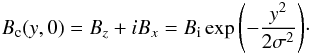 (6)Our complex variable can
be interpreted as a Fourier integral, evolving in time as:
(6)Our complex variable can
be interpreted as a Fourier integral, evolving in time as: 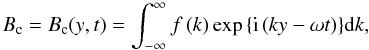 (7)with
f(k) determined by the initial conditions:
(7)with
f(k) determined by the initial conditions:
 (8)where we have used the
standard result (Abramowitz & Stegun 1964,
Eq. (7.4.6)):
(8)where we have used the
standard result (Abramowitz & Stegun 1964,
Eq. (7.4.6)):  (9)We also use this result
to evaluate the integral in Eq. (7) in the
limit , finding:
(9)We also use this result
to evaluate the integral in Eq. (7) in the
limit , finding: ![\begin{equation} B_{\rm c}=\sum_{+,-}\frac{B_{\rm i}}{{\sqrt{1+\left(\frac{\eta}{\muo}-{\rm i}\ca\di \right)\frac{t}{\sigma^2} }}} {\exp{\left( \frac{-\left(y\pm\ca t \right)^2}{2\left[\sigma^2+\left(\frac{\eta}{\muo}-{\rm i}\ca\di\right)t\right] }\right) }} \label{eq:B_c(y,t)} \end{equation}](/articles/aa/full_html/2011/01/aa15479-10/aa15479-10-eq52.png) (10)where
the summation is over forward- and backward-propagating waves. Equation (10) describes a pair of pulses travelling in
opposite direction at approximately the Alfvén speed, which are damped by finite
resistivity and circularly polarised. We can also calculate the contribution to the total
energy per unit area in (x, z),
ℰBTOT, made by the magnetic energy per unit
area in (x, z) of both pulses
(ℰBc) as follows:
(10)where
the summation is over forward- and backward-propagating waves. Equation (10) describes a pair of pulses travelling in
opposite direction at approximately the Alfvén speed, which are damped by finite
resistivity and circularly polarised. We can also calculate the contribution to the total
energy per unit area in (x, z),
ℰBTOT, made by the magnetic energy per unit
area in (x, z) of both pulses
(ℰBc) as follows:
 Since the magnetic
perturbation is transverse to the equilibrium field,
B0·B1 = 0
and hence
Since the magnetic
perturbation is transverse to the equilibrium field,
B0·B1 = 0
and hence  (11)Many of the factors
in
(11)Many of the factors
in  will cancel
upon integration, hence the energy associated with the pulse
(ℰBc) evolves as:
will cancel
upon integration, hence the energy associated with the pulse
(ℰBc) evolves as: 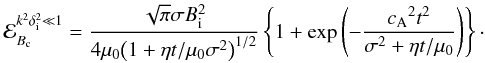 (12)Thus after a short
initial transient phase (essentially the time taken for an Alfvén wave to travel a
distance equal to the initial pulse width, σ), we recover a power law
decay (∝t −1/2 for
t ≫ μ0σ2 / η)
in the energy associated with the pulse. This expression (Eq. (12)) is compared with several numerical
simulation results in Sect. 3, and can be seen in
Fig. 2. It is straightforward to show that the
expression given by Eq. (12) for the Hall
MHD long wavelength () regime is identical
to that found for an initially Gaussian pulse in the MHD limit.
(12)Thus after a short
initial transient phase (essentially the time taken for an Alfvén wave to travel a
distance equal to the initial pulse width, σ), we recover a power law
decay (∝t −1/2 for
t ≫ μ0σ2 / η)
in the energy associated with the pulse. This expression (Eq. (12)) is compared with several numerical
simulation results in Sect. 3, and can be seen in
Fig. 2. It is straightforward to show that the
expression given by Eq. (12) for the Hall
MHD long wavelength () regime is identical
to that found for an initially Gaussian pulse in the MHD limit.
2.2. Short wavelength Hall MHD regime (uniform)
Turning to the opposite limit, , the perturbation
frequencies (5b) comprise of a
combination of resistively damped whistler and ion cyclotron waves. We can again describe
the pulse evolution associated with each separate wave branch in this limit, in the manner
described previously (Sect. 2.1), again for an
initially Gaussian perturbation. Beginning with (7), and with the same initial conditions (8) as the previous limit, we find that the whistler wave calculation
proceeds similarly to that of the previous section, however the i.c. wave (being
independent of wavenumber) differs somewhat: 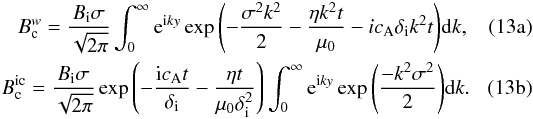 Evaluating
the integrals in Eq. (13b), using
Eq. (9), we obtain:
Evaluating
the integrals in Eq. (13b), using
Eq. (9), we obtain: ![\begin{subequations} \begin{eqnarray} \label{eq:Bcw2} B_{\rm c}^{w}\!=\!\frac{B_{\rm i}}{{\sqrt{1+2\left(\frac{\eta}{\muo}-{\rm i}\ca\di \right)\frac{t}{\sigma^2} }}} {\exp{\left( \frac{-y^2}{2\left[\sigma^2+2\left(\frac{\eta}{\muo}-{\rm i}\ca\di\right)t\right] }\right) }} \\ \label{eq:Bcic2} B_{\rm c}^{\rm ic}=B_{\rm i}\exp{\left(-\frac{ {\rm i}\ca t}{\di}-\frac{\eta t}{\muo\di^2} \right) } \exp{\left(-\frac{y^2}{2\sigma^2} \right) }\cdot \end{eqnarray} \label{eq:Bclarge} \end{subequations}](/articles/aa/full_html/2011/01/aa15479-10/aa15479-10-eq66.png) In
this short wavelength () regime, the peak of the pulse
now no longer propagates, but decreases in amplitude. The right circularly polarised
component of the pulse rapidly broadens, due to the high whistler speed, and damps
algebraically at a rate similar to that found in both the MHD and long wavelength
(
In
this short wavelength () regime, the peak of the pulse
now no longer propagates, but decreases in amplitude. The right circularly polarised
component of the pulse rapidly broadens, due to the high whistler speed, and damps
algebraically at a rate similar to that found in both the MHD and long wavelength
( ) Hall
MHD regimes. The left circularly polarised (ion cyclotron wave) component, on the other
hand, damps exponentially. It should be noted that this damping arises from resistive
dissipation, and as such should be distinguished from the kinetic ion cyclotron damping
arising from wave-particle interactions.
) Hall
MHD regimes. The left circularly polarised (ion cyclotron wave) component, on the other
hand, damps exponentially. It should be noted that this damping arises from resistive
dissipation, and as such should be distinguished from the kinetic ion cyclotron damping
arising from wave-particle interactions.
We may, again, calculate the energy associated with each solution (14b), using (11), where we still only obtain transverse perturbations, and hence
B1·B0
still makes no contribution to the energy. In this limit, we obtain an expression for the
energy associated with the individual whistler and i.c. wave branches: 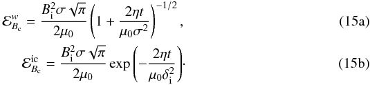 Thus,
for waves in the regime, we no longer see the
initial transient phase seen previously in (12), and for long timescales the algebraically-damped whistler contribution to
the wave energy is dominant over the exponentially-damped contribution from the ion
cyclotron wave.
Thus,
for waves in the regime, we no longer see the
initial transient phase seen previously in (12), and for long timescales the algebraically-damped whistler contribution to
the wave energy is dominant over the exponentially-damped contribution from the ion
cyclotron wave.
2.3. Phase-mixing and damping in a non-uniform plasma
By now allowing the equilibrium plasma density to vary in a direction perpendicular to
both the direction of the equilibrium field (y) and the direction of
initial perturbation (z), we can investigate what effect the Hall term
has on the dissipation rate in a non-uniform plasma. When the gradients in the
x-direction are sufficiently large, and the effects of viscosity are
negligible, the linearised Alfvén wave equation in the MHD limit takes the form (Hood et al. 2002): 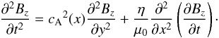 (16)The
variation in Alfvén speed
(16)The
variation in Alfvén speed  causes steep gradients to build up in the direction of the inhomogeneity which, in turn,
significantly enhances resistive damping in the regions where the inhomogeneity is
greatest. Hood et al. (2002) used a multiple
time-scale analysis to derive from Eq. (16) a one-dimensional diffusion equation whose solutions can be expressed in terms
of the Alfvén speed gradient
cA′(x) = dcA(x) / dx.
For the case of the initially Gaussian pulse defined by Eq. (6), the forward-propagating solution takes the form:
causes steep gradients to build up in the direction of the inhomogeneity which, in turn,
significantly enhances resistive damping in the regions where the inhomogeneity is
greatest. Hood et al. (2002) used a multiple
time-scale analysis to derive from Eq. (16) a one-dimensional diffusion equation whose solutions can be expressed in terms
of the Alfvén speed gradient
cA′(x) = dcA(x) / dx.
For the case of the initially Gaussian pulse defined by Eq. (6), the forward-propagating solution takes the form: ![\begin{equation} B_z=\frac{B_{\rm i}}{2\sqrt{1+\ca'^2\eta t^3/3\muo\sigma^2}}\exp{\left(-\frac{\left(y-\ca t\right)^2 }{2\left[\sigma^2+\ca'^2\eta t^3/3\muo\right] }\right) }\cdot \label{eq:Hood1} \end{equation}](/articles/aa/full_html/2011/01/aa15479-10/aa15479-10-eq74.png) (17)We can evaluate the
perturbed magnetic field energy per unit length in the z-direction
(17)We can evaluate the
perturbed magnetic field energy per unit length in the z-direction
 for this case
by integrating
for this case
by integrating  over a finite
distance
x0 < x < x1
in the x-direction and from minus to plus infinity in the
y-direction, taking into account the presence of both forward- and
backward-propagating pulses. The y-integration can be performed
analytically, yielding:
over a finite
distance
x0 < x < x1
in the x-direction and from minus to plus infinity in the
y-direction, taking into account the presence of both forward- and
backward-propagating pulses. The y-integration can be performed
analytically, yielding: 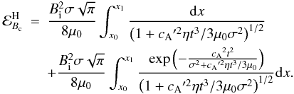 (18)The
integrals in this expression can be readily evaluated numerically, to allow comparison
with our numerical simulations in the next section.
(18)The
integrals in this expression can be readily evaluated numerically, to allow comparison
with our numerical simulations in the next section.
3. Simulation results
The system was modelled numerically using a two dimensional version of a Lagrangian remap
scheme (LareXd), described by Arber et al. (2001),
which includes an optional Hall physics package to incorporate the Hall term into the
standard MHD system of equations, seen here in normalised dimensionless form:
![\begin{eqnarray*} &&\frac{\partial \rho}{\partial t}+\dive{\left(\rho{\vec{v}} \right) }=0, \\ &&\rho\left( \frac{\partial {\vec{v}}}{\partial t}+\left( {\vec{v}}\cdot\boldnabla\right){\vec{v}} \right)= \left(\curl{\vec{B}}\right)\times{\vec{B}}-\grad{p}, \\ &&\frac{\partial {\vec{B}}}{\partial t}=\curl{\left( {\vec{v}}\times{\vec{B}}\right) }-\curl{\left(\eta\curl{\vec{B}} \right) } -\lambda_{\rm i}\curl{\left[\frac{1}{\rho}\left(\curl{\vec{B}}\times{\vec{B}} \right) \right] }, \\ &&\rho\left( \frac{\partial\epsilon}{\partial t}+\left( {\vec{v}}\cdot{\boldnabla}\right)\epsilon\right) =-p\dive{\vec{v}}+\eta j^2, \end{eqnarray*}](/articles/aa/full_html/2011/01/aa15479-10/aa15479-10-eq79.png) for
dimensionless mass density ρ, pressure p, magnetic field
strength B, fluid
velocity v, internal energy density ϵ,
resistivity η (the reciprocal of the Lundquist number) and ion skin depth
λi( = δi / l0).
for
dimensionless mass density ρ, pressure p, magnetic field
strength B, fluid
velocity v, internal energy density ϵ,
resistivity η (the reciprocal of the Lundquist number) and ion skin depth
λi( = δi / l0).
In Sect. 1, two particular regimes were identified where collisional models, such as this, may be more appropriate to describe the plasma behaviour than collisionless treatments. Normalising temperatures (T0) and densities (n0) using flaring coronal values (T0 ≈ 2 × 10⁶ K and n0 ≈ 1016 m-3) or upper chromospheric values (T0 ≈ 2 × 10⁴ K and n0 ≈ 2 × 10¹⁶ m-3) places the simulations firmly within these regimes. Specifying a low plasma beta (β = 0.01) in the simulations fixes the normalising magnetic field strengths to B0 ≈ 118 G in the flaring corona, or B0 ≈ 17 G in the upper chromosphere. This also determines the effective size of several fundamental plasma parameters, outlined for these normalising values in Table 1.
Approximate lengthscales.
The parameter λi (which controls the effect of the Hall term in
our simulations) was initially set equal to 0.0072. Using this value
of λi, together with the ion skin depths listed in Table 1, implies a normalising lengthscale
l0 = 0.3 km in the flaring corona, and
l0 = 0.2 km in the chromosphere. Given that the mean square
wavenumber for a Gaussian pulse of width σ can be found using
⟨ k2 ⟩ = 1 / σ2, a choice of
width σ = 0.1 places the simulations firmly within the long wavelength
regime (discussed in Sect. 2.1), as
 . By relating simulated perturbation
frequencies (ω) to the perturbation size (by assuming
ω ~ kcA), our
choices for λi and σ perturb the simulations
with frequencies which have begun to approach the ion cyclotron frequency
(ω / Ωi ~ kδi ~ λi / σ ~ 0.07).
. By relating simulated perturbation
frequencies (ω) to the perturbation size (by assuming
ω ~ kcA), our
choices for λi and σ perturb the simulations
with frequencies which have begun to approach the ion cyclotron frequency
(ω / Ωi ~ kδi ~ λi / σ ~ 0.07).
As pointed out by Craig & Litvinenko (2002), the resistivity could be as much as a factor of 106 higher than the classical Spitzer value in the flaring corona. Using this enhancement factor and the normalisation described above for flaring conditions, we find η = 0.0005. Note that using the same value for η and the chromospheric normalisation, the enhancement of the resistivity as compared to the Spitzer value, is less than 102. An enhancement in the resistivity implies a corresponding reduction of the mean free paths quoted in Table 1. These reduced mean free paths are then much smaller than the typical wavelengths of the modes under consideration, so that Hall MHD is an appropriate model to use.
In order to study phase-mixing, we allow the equilibrium density to vary
along x, with the form:  (19)chosen for constant density
at the edges, ρ(0) = ρ(1) = 1, and a central increase in
density controlled by a steepness parameter, α. We also vary the specific
internal energy density of the system, ϵ, allowing us to define a constant
plasma pressure in terms of the plasma beta, β( = 0.01), and the magnetic
pressure, as:
(19)chosen for constant density
at the edges, ρ(0) = ρ(1) = 1, and a central increase in
density controlled by a steepness parameter, α. We also vary the specific
internal energy density of the system, ϵ, allowing us to define a constant
plasma pressure in terms of the plasma beta, β( = 0.01), and the magnetic
pressure, as:
 We set up a constant
equilibrium field to reflect the analytical setup, with
B0( = [ B0x,B0y,B0z ] ) = [ 0,1,0 ] ,
which we perturb in the form outlined by Eq. (6). As our analytical work is based on a linearised system of equations, we fix
the pulse amplitude, Bi( = 0.0005) to be small enough that we
minimise non-linear effects. A 2000 × 2000 grid was used to fully resolve the effects of a
density gradient in x and potential whistler/i.c. effects
in y. As the density and energy density profiles are symmetric, periodic
boundary conditions are used in x, whilst the y boundaries
are left open, and the simulation terminated before the pulse reaches the boundaries. The
range of the numerical box (set, for the simulations, at
− 10 ≤ y ≤ 10, 0 ≤ x ≤ 1) has a large range
in y, in anticipation of the pulse propagation.
We set up a constant
equilibrium field to reflect the analytical setup, with
B0( = [ B0x,B0y,B0z ] ) = [ 0,1,0 ] ,
which we perturb in the form outlined by Eq. (6). As our analytical work is based on a linearised system of equations, we fix
the pulse amplitude, Bi( = 0.0005) to be small enough that we
minimise non-linear effects. A 2000 × 2000 grid was used to fully resolve the effects of a
density gradient in x and potential whistler/i.c. effects
in y. As the density and energy density profiles are symmetric, periodic
boundary conditions are used in x, whilst the y boundaries
are left open, and the simulation terminated before the pulse reaches the boundaries. The
range of the numerical box (set, for the simulations, at
− 10 ≤ y ≤ 10, 0 ≤ x ≤ 1) has a large range
in y, in anticipation of the pulse propagation.
Our initial investigation sought to recover, using Lare2d, the behaviour of the pulse and its evolution along the equilibrium field, in the long wavelength Hall MHD regime (expressed in Eq. (10)). For this investigation, selecting a steepness factor of α = 0 in our equilibrium density expression (Eq. (19)) provided the required uniform equilibrium density and uniform internal energy in the simulations. We found that the evolution of the pulse in the numerical scheme exactly matched the equivalent analytical expression (Eq. (10)), both in the MHD and long-wavelength Hall MHD (λi = 0.0072) limits.
Density enhancement values.
Moving to the non-uniform equilibrium density simulations, we then selected a range of specific equilibrium density enhancements through the steepness parameter α according to Eq. (19). The specific values of α chosen, and the corresponding density enhancements are listed in Table 2.
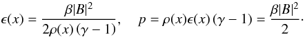
As discussed previously, Hood et al. (2002) obtained an expression describing the evolution of a pulse as it undergoes phase mixing in the MHD limit (Eq. (17)). We sought to test the validity of this expression for a range of equilibrium density gradients using Lare2d, by tracking the height and location of the peak of the pulse as it travelled along the equilibrium field, and comparing this with the pulse amplitude damping rate found by Hood et al. (2002). We found that the MHD simulations with large equilibrium density increases displayed good agreement with the proposed damping rate, but this agreement was lessened by reducing the equilibrium density enhancement. Furthermore, we repeated the simulations for the long wavelength Hall MHD regime, again finding that the amplitude evolution of the pulse was in agreement with the expression proposed by Hood et al. (2002), but only in the cases where the density enhancement was sufficiently large. These results are summarised in Fig. 1.
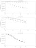 |
Fig. 1 Comparison of predicted amplitude fall-off for an analytical treatment of MHD phase-mixing (Eq. (17) – solid curve), with tracked pulse peak of Lare2d simulations. Displayed are the results of the MHD (crosses) and long wavelength Hall MHD (diamonds) simulations for three different density gradients (for corresponding density enhancements, see Table 2). |
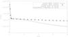 |
Fig. 2 Temporal evolution of magnetic energy perturbation associated with initially Gaussian pulse, computed analytically for cases with uniform equilibrium density using Eq. (11) (stars), and strong equilibrium density gradient using Eq. (18) (dotted curve). The solid and dashed curves show the corresponding numerical results, obtained using Lare2d. |
Having studied the behaviour of the perturbed magnetic energy evolution in the uniform and steep density gradient limits using MHD simulations, we then investigated the energy response for a variety of different density gradients, and at different skin depths. For clarity, we also included the perturbed internal energy evolution of the pulse. Our first set of results compare the evolution of the pulse in MHD, with that of the λi = 0.0072 simulations, corresponding to the long wavelength Hall MHD regime, discussed in Sect. 2.1. These results are seen in Fig. 3.
Figure 3 clearly displays differences between the MHD and Hall MHD cases, for density gradients which are neither uniform nor very steep. To gain insight into the reasons for these differences, we have also tracked the evolution of the pulse profile in the x-direction as it travels at the Alfvén speed of the steepest density region. In the Hall MHD cases, we observe consistently smaller amplitude gradients. As an example of this, Fig. 4 shows snapshots of MHD and Hall MHD pulse profiles in simulations with α = 5 / 18. One might have expected the dispersive effects of the Hall term to induce a cascade into short wavelengths, which could in principle invalidate our neglect of kinetic effects. However, Fig. 4 shows that the opposite effect occurs: the Hall term actually reduces the gradients resulting from phase mixing.
We have demonstrated analytically that the plasma response dramatically differs in the
short wavelength () Hall MHD limit, from that of the
MHD and long wavelength Hall MHD limits (Sect. 2). Our
final investigation sought to begin to bring out the behaviour of this limit by increasing
λi by a factor of 10. In doing so, we also reduce the
associated enhancement factor in resistivity required to justify setting
η = 0.0005 in the code. The enhancement factor is reduced to 105
for the flaring corona, whilst for the upper chromosphere the effective resistivity is less
than an order of magnitude larger than the equivalent Spitzer value, using the values
outlined earlier in Sect. 3. In these simulations, we
also increased the size of the numerical box (to − 30 ≤ y ≤ 30,
0 ≤ x ≤ 1, accounting for larger dispersive effects and the faster
whistler wave component) and the number of gridpoints (now at 6000 × 2000, maintaining the
same resolution). The perturbed frequencies in these simulations are now a large fraction of
the ion cyclotron frequency
(ω / Ωi ~ λi/σ ~ 0.7).
Figure 5 compares the response of the perturbed
magnetic and internal energies in simulations of a Hall MHD plasma with
λi = 0.072, with that of an MHD plasma, for three density
gradient cases which are neither uniform, nor dramatically varying. It is clear that in this
Hall MHD regime, there is a strong reduction in the damping rate compared to the MHD limit.
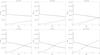 |
Fig. 3 Evolution of field perturbation energy in MHD (solid curve) and λi = 0.0072 Hall MHD (dashed curve) simulations for six values of density steepness parameter α. The internal energy is also plotted for the MHD (dot-dash curve) and λi = 0.0072 Hall MHD (dotted curve) simulations. |
4. Discussion and conclusions
The behaviour demonstrated by the analysis of a uniform plasma in the long wavelength Hall MHD regime (Sect. 2.1) was fully recovered by the Lare2d simulations. Both the simulated pulse evolution and its associated magnetic energy are indistinguishable from the expressions derived analytically (Eq. (10) and Eq. (11) respectively). The simulations show that the MHD results remain linearly polarised, whilst the long wavelength Hall MHD pulse becomes circularly polarised. However, both the simulations and the analytical results tell us that this has no impact on the magnetic energy associated with the pulse, which damps at the same rate in both regimes.
Considering now the results of the investigation concerning a non-uniform equilibrium
density, Fig. 1 shows that the amplitude damping rate
described by Hood et al. (2002) is well matched to
the rate of damping of the peak of an MHD pulse when the gradient in Alfvén speed is
sufficiently steep. Whilst not a particularly surprising result, as the strong phase mixing
limit required for Eq. (16) to be valid
applies in this case, it is somewhat more surprising to find for sufficiently steep Alfvén
speed gradients, that the long wavelength Hall MHD regime also conforms to this amplitude
damping rate. For shallower gradients in Alfvén speed, Fig. 1 also demonstrates that this damping rate quickly becomes inappropriate for the
Hall MHD simulations, whilst giving
better agreement with the MHD evolution of the peak of the pulse. This is partly due to the
fact that in the Hall regime, the pulse is no longer linearly polarised, quickly losing
amplitude to the other field components. The Hall regime is also subject to significant
dispersive effects, which reduce the amplitude of the pulse as it spreads along the
equilibrium field. However, for sufficiently steep density gradients, phase-mixing becomes
the dominant cause of amplitude dissipation.
By comparing the energy evolution associated with our numerical simulations of an MHD pulse to that found by numerically integrating an expression for the pulse evolution given by Hood et al. (2002) in Fig. 2, we see that, apart from a slight initial delay, the two results appear closely matched. The reason for the difference between the two is simply due to the treatments used. The linearised Alfvén wave (Eq. (16)) used in the treatments of Heyvaerts & Priest (1983) and Hood et al. (2002) retains only the x-derivatives, on the basis that derivatives along the field are small compared to those across it. However, in our simulations, the (initially uniform) pulse propagates a finite distance in which the y-derivative causes resistive damping along the equilibrium field. This continues until the gradients in x build up sufficiently to allow phase-mixing to become the dominant damping mechanism. The brief initial period of longitudinal damping is not included in the treatment of Hood et al. (2002), resulting in the discrepancies in behaviour seen between the energy evolution of the two non-uniform scenarios shown in Fig. 2.
Our final investigation sought to compare the response of the magnetic and internal energies associated with the pulse for different equilibrium density gradients and at different skin-depths. Figure 3 shows that for shallow density gradients, both MHD and long wavelength Hall MHD simulations display similar behaviour to that seen in the uniform case. For the steepest density gradients considered, again the long wavelength Hall MHD and MHD simulations exhibit similar behaviour, suggesting that MHD phase-mixing dominates the energy evolution (see Fig. 2). However, we see significant departures from the MHD behaviour of both perturbed magnetic and internal energies associated with the long wavelength Hall MHD regime, in the cases where the density is neither uniform nor sharply varying. In these cases, the inclusion of the Hall term causes the damping rate of perturbed magnetic energy to be reduced. Consequently there is a slower increase in the internal energy of the pulse than that seen in MHD: phase-mixing of the plasma causes less rapid plasma heating in the Hall MHD regime than in the MHD regime.
Evidence to support this can be seen in Fig. 4, where we plot a slice (in x) through pulse amplitude at the location (along y) of maximum phase-mixing, both for the λi = 0.0072 and MHD simulations. The figure clearly demonstrates that in the Hall case, the gradients in x are smaller than those in the MHD case. The whistler component of the Hall MHD pulse displays highly dispersive behaviour, which increases with skin depth. This dispersion spreads the pulse envelope along the equilibrium field as it travels, introducing higher wavenumbers into the pulse but only in the equilibrium field direction. In the density gradient direction, the group dispersion of the wave has the effect of reducing the damping rate by making amplitude gradients across the field (in x) smaller, reducing the efficiency of phase-mixing and its damping of the magnetic energy of the pulse.
This behaviour is also seen in the higher skin depth Hall MHD simulations. In the λi = 0.072 simulation results, seen in Fig. 5, there is now a very significant reduction in the damping rate of the magnetic energy, even in the steep density gradient case, which, in the long wavelength Hall MHD regime has begun to converge to the MHD results. As the skin depth is increased, the equilibrium density gradient must also be increased in order to recover a rate of energy dissipation comparable to those seen in the long wavelength Hall MHD and MHD limits.
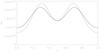 |
Fig. 4 Comparison of two snapshots of slices (in x) through the pulse amplitude, at location (in y) of maximum phase-mixing. Snapshots shown are for long wavelength Hall MHD (solid) and MHD (dashed) cases, taken at the same time, for an identical initial pulse and with density steepness α = 5 / 18. |
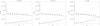 |
Fig. 5 Evolution of field perturbation energy in MHD (solid curve) and λi = 0.072 Hall MHD (stars) simulations for three intermediate values of density gradient parameter α. Also plotted is the internal energy for the MHD (dot-dash curve) and λi = 0.072 Hall MHD (crosses) simulations. |
In summary, we have described analytically the propagation of an initially Gaussian field perturbation along a uniform equilibrium field in the presence of resistivity, and the evolution of magnetic energy associated with this perturbation. While the evolution of the perturbation differs in the MHD, long wavelength and short wavelength Hall MHD regimes, the energy evolution is the same in the MHD and long wavelength Hall MHD cases. In a non-uniform equilibrium plasma, our simulations show that the damping rate for the energy associated with the pulse in Hall MHD is significantly reduced when the Alfvén speed variation is neither uniform nor sharply varying, compared to that of an MHD treatment as the Hall term actually reduces the gradients resulting from phase-mixing. Moreover, as the ion skin depth is increased, the density gradient needed for MHD phase-mixing to dominate the evolution of the pulse (the “strong phase-mixing limit”) must also increase.
Acknowledgments
This work was funded by the United Kingdom Engineering and Physical Sciences Research Council, under grant EP/G003955 and a CASE studentship, and by the European Communities under the contract of Association between EURATOM and CCFE. The views and opinions expressed herein do not necessarily reflect those of the European Commission. We thank P. J. Cargill & T. Neukirch (University of St. Andrews) for helpful discussions. I.D.M. acknowledges support of a Royal Society University Research Fellowship.
References
- Abramowitz, M., & Stegun, I. A. 1964, Handbook of Mathematical Functions with Formulas, Graphs, and Mathematical Tables (New York: Dover) [Google Scholar]
- Arber, T. D., Longbottom, A. W., Gerrard, C. L., & Milne, A. M. 2001, J. Comput. Phys., 171, 151 [NASA ADS] [CrossRef] [Google Scholar]
- Bian, N., & Kontar, E. 2010, A&A, submitted [arXiv:1006.2729] [Google Scholar]
- Birn, J., & Priest, E. 2007, Reconnection of Magnetic Fields (New York: Cambridge University Press), 94 [Google Scholar]
- Birn, J., Drake, J. F., Shay, M. A., et al. 2001, J. Geophys. Res., 106, 3715 [Google Scholar]
- Botha, G. J. J., Arber, T. D., Nakariakov, V. M., & Keenan, F. P. 2000, A&A, 363, 1186 [NASA ADS] [Google Scholar]
- Craig, I. J. D., & Litvinenko, Y. E. 2002, ApJ, 570, 387 [NASA ADS] [CrossRef] [Google Scholar]
- Craig, I. J. D., Litvinenko, Y. E., & Senanayake, T. 2005, A&A, 433, 1139 [NASA ADS] [CrossRef] [EDP Sciences] [Google Scholar]
- De Moortel, I. 2009, Space Sci. Rev., 149, 65 [NASA ADS] [CrossRef] [Google Scholar]
- De Moortel, I., Hood, A. W., Ireland, J., & Arber, T. D. 1999, A&A, 346, 641 [NASA ADS] [Google Scholar]
- De Moortel, I., Hood, A. W., & Arber, T. D. 2000, A&A, 354, 334 [NASA ADS] [Google Scholar]
- Génot, V., Louarn, P., & Mottez, F. 2004, Ann. Geophys., 22, 2081 [NASA ADS] [CrossRef] [Google Scholar]
- Hamilton, B., McClements, K. G., Fletcher, L., & Thyagaraja, A. 2003, Sol. Phys., 214, 339 [NASA ADS] [CrossRef] [Google Scholar]
- Heyvaerts, J., & Priest, E. R. 1983, A&A, 117, 220 [NASA ADS] [Google Scholar]
- Hood, A. W., Ireland, J., & Priest, E. R. 1997, A&A, 318, 957 [NASA ADS] [Google Scholar]
- Hood, A. W., Brooks, S. J., & Wright, A. N. 2002, R. Soc. London Proc. Ser. A, 458, 2307 [Google Scholar]
- Marsch, E. 2006, Liv. Rev. Sol. Phys., 3, 1 [Google Scholar]
- Nakariakov, V. M., Roberts, B., & Murawski, K. 1997, Sol. Phys., 175, 93 [NASA ADS] [CrossRef] [Google Scholar]
- Ono, M., & Kulsrud, R. M. 1975, Phys. Fluids, 18, 1287 [NASA ADS] [CrossRef] [Google Scholar]
- Parker, E. N. 1991, ApJ, 376, 355 [NASA ADS] [CrossRef] [Google Scholar]
- Sckopke, N., Paschmann, G., Brinca, A. L., Carlson, C. W., & Luehr, H. 1990, J. Geophys. Res., 95, 6337 [NASA ADS] [CrossRef] [Google Scholar]
- Tsiklauri, D., & Haruki, T. 2008, Phys. Plasmas, 15, 112902 [NASA ADS] [CrossRef] [Google Scholar]
- Tsiklauri, D., Sakai, J.-I., & Saito, S. 2005, A&A, 435, 1105 [NASA ADS] [CrossRef] [EDP Sciences] [Google Scholar]
All Tables
All Figures
|
Fig. 1 Comparison of predicted amplitude fall-off for an analytical treatment of MHD phase-mixing (Eq. (17) – solid curve), with tracked pulse peak of Lare2d simulations. Displayed are the results of the MHD (crosses) and long wavelength Hall MHD (diamonds) simulations for three different density gradients (for corresponding density enhancements, see Table 2). |
| In the text | |
|
Fig. 2 Temporal evolution of magnetic energy perturbation associated with initially Gaussian pulse, computed analytically for cases with uniform equilibrium density using Eq. (11) (stars), and strong equilibrium density gradient using Eq. (18) (dotted curve). The solid and dashed curves show the corresponding numerical results, obtained using Lare2d. |
| In the text | |
|
Fig. 3 Evolution of field perturbation energy in MHD (solid curve) and λi = 0.0072 Hall MHD (dashed curve) simulations for six values of density steepness parameter α. The internal energy is also plotted for the MHD (dot-dash curve) and λi = 0.0072 Hall MHD (dotted curve) simulations. |
| In the text | |
|
Fig. 4 Comparison of two snapshots of slices (in x) through the pulse amplitude, at location (in y) of maximum phase-mixing. Snapshots shown are for long wavelength Hall MHD (solid) and MHD (dashed) cases, taken at the same time, for an identical initial pulse and with density steepness α = 5 / 18. |
| In the text | |
|
Fig. 5 Evolution of field perturbation energy in MHD (solid curve) and λi = 0.072 Hall MHD (stars) simulations for three intermediate values of density gradient parameter α. Also plotted is the internal energy for the MHD (dot-dash curve) and λi = 0.072 Hall MHD (crosses) simulations. |
| In the text | |
Current usage metrics show cumulative count of Article Views (full-text article views including HTML views, PDF and ePub downloads, according to the available data) and Abstracts Views on Vision4Press platform.
Data correspond to usage on the plateform after 2015. The current usage metrics is available 48-96 hours after online publication and is updated daily on week days.
Initial download of the metrics may take a while.