| Issue |
A&A
Volume 520, September-October 2010
|
|
|---|---|---|
| Article Number | A28 | |
| Number of page(s) | 16 | |
| Section | Numerical methods and codes | |
| DOI | https://doi.org/10.1051/0004-6361/201014700 | |
| Published online | 24 September 2010 | |
Test-field method for mean-field coefficients with MHD background
M. Rheinhardt1 - A. Brandenburg1,2
1 -
NORDITA, AlbaNova University Center, Roslagstullsbacken 23,
10691 Stockholm, Sweden
2 -
Department of Astronomy, AlbaNova University Center,
Stockholm University, 10691 Stockholm, Sweden
Received 1 April 2010 / Accepted 27 May 2010
Abstract
Aims. The test-field method for computing turbulent
transport coefficients from simulations of hydromagnetic flows is
extended to the regime with a magnetohydrodynamic (MHD) background.
Methods. A generalized set of test equations is derived using
both the induction equation and a modified momentum equation. By
employing an additional set of auxiliary equations, we obtain linear
equations describing the response of the system to a set of prescribed
test fields. Purely magnetic and MHD backgrounds are emulated by
applying an electromotive force in the induction equation analogously
to the ponderomotive force in the momentum equation. Both forces are
chosen to have Roberts-flow like geometry.
Results. Examples with purely magnetic as well as MHD
backgrounds are studied where the previously used quasi-kinematic
test-field method breaks down. In cases with homogeneous mean fields it
is shown that the generalized test-field method produces the same
results as the imposed-field method, where the field-aligned component
of the actual electromotive force from the simulation is used.
Furthermore, results for the turbulent diffusivity are given, which are
inaccessible to the imposed-field method. For MHD backgrounds, new
mean-field effects are found that depend on the occurrence of
cross-correlations between magnetic and velocity fluctuations. In
particular, there is a contribution to the mean Lorentz force that is
linear in the mean field and hence reverses sign upon a reversal of the
mean field. For strong mean fields, ![]() is found to be quenched proportional to the fourth power of the field strength, regardless of the type of background studied.
is found to be quenched proportional to the fourth power of the field strength, regardless of the type of background studied.
Key words: magnetohydrodynamics - dynamo - Sun: dynamo - stars: magnetic field - methods: numerical
1 Introduction
Astrophysical bodies such as stars with outer convective envelopes,
accretion discs, and galaxies tend to be magnetized.
In all those cases the magnetic field varies on a broad spectrum of scales.
On small scales the magnetic field might well be the result of scrambling an
existing large-scale field by a small-scale flow.
However, at large magnetic Reynolds numbers, i.e. when advection dominates
over magnetic diffusion, another source of small-scale fields is
small-scale dynamo action (Kazantsev 1968).
This process is now fairly well understood and confirmed by numerous
simulations (Cho & Vishniac 2000; Schekochihin et al. 2002,
2004; Haugen et al. 2003, 2004); for a review see Brandenburg & Subramanian (2005).
Especially in the context of magnetic fields of galaxies, the
occurrence of small-scale dynamos
may be important for providing a strong
field on short time scales (
![]() ), which may then act as
the seed for a large-scale dynamo (Beck et al. 1994).
), which may then act as
the seed for a large-scale dynamo (Beck et al. 1994).
In contemporary galaxies the strength of magnetic fields on small and large length scales is comparable (Beck et al. 1996), but in stars this is less clear. On the solar surface the solar magnetic field shows significant energy in small scales. (Solanki et al. 2006). The possibility of generating such magnetic fields locally in the upper layers of the convection zone by a small-scale dynamo is sometimes referred to as surface dynamo (Cattaneo 1999; Emonet & Cattaneo 2001; Vögler & Schüssler 2007). On the other hand, simulations of stratified convection with shear show that small-scale dynamo action is a prevalent feature of the kinematic regime, but becomes less important when the field is strong and saturated (Brandenburg 2005a; Käpylä et al. 2008).
An important question is then how the primary
presence of small-scale magnetic fields affects
the generation of large-scale fields
if these are the result of a large-scale dynamo.
Such a process creates
magnetic fields on scales large compared with those of the
energy-carrying eddies of the underlying, in general turbulent flow
via an instability (Parker 1979).
A commonly used tool for studying this type of dynamos is mean-field
electrodynamics, where correlations of small-scale magnetic and velocity
fields are expressed in terms of the mean magnetic field and the mean velocity using
corresponding turbulent transport coefficients or their associated integral kernels
(Moffatt 1978; Krause & Rädler 1980).
The determination of these coefficients
(e.g., ![]() effect and turbulent diffusivity)
is the central task of mean-field dynamo theory.
This can be performed analytically, but usually only via approximations
which are hardly justified in realistic astrophysical situations
where the magnetic Reynolds numbers,
effect and turbulent diffusivity)
is the central task of mean-field dynamo theory.
This can be performed analytically, but usually only via approximations
which are hardly justified in realistic astrophysical situations
where the magnetic Reynolds numbers,
![]() ,
are large.
,
are large.
Obtaining turbulent transport coefficients from direct numerical simulations (DNS) offers a more sustainable alternative as it avoids the restricting approximations and uncertainties of analytic approaches. Moreover, no assumptions concerning correlation properties of the turbulence need to be made, because a direct ``measurement'' of those properties is performed in a physically consistent situation emulated by the DNS. The simplest way to accomplish such a measurement is to include an imposed large-scale magnetic field in the DNS, whose influence on the fluctuations of magnetic field and velocity is utilized in inferring a subset of the relevant transport coefficients. We refer to this technique as the imposed-field method. As an important limitation, it has to be required that the actual mean field in the main run, which may differ from the initially imposed one, is uniform. Otherwise the results will be corrupted (Käpylä et al. 2010).
A more universal tool is offered by the test-field method (Schrinner et al. 2005, 2007), which allows the determination of all wanted transport coefficients from a single DNS. For this purpose the fluctuating velocity is taken from the DNS and inserted into a properly tailored set of test equations. Their solutions, the test solutions, represent fluctuating magnetic fields as responses to the interaction of the fluctuating velocity with a set of suitably chosen mean fields, the test fields. For distinction from the test equations, which are in general also solved by direct numerical simulation, we will refer to the original DNS as the main run. This method has been successfully applied to homogeneous turbulence with helicity (Sur et al. 2008; Brandenburg et al. 2008a), with shear and no helicity (Brandenburg et al. 2008b), and with both (Mitra et al. 2009).
A crucial requirement on any test-field method is the independence of the resulting transport coefficients on the strength and geometry of the test fields. This is immediately plausible in the kinematic situation, i.e., if there is no back-reaction of the mean magnetic field on the flow. Indeed, for given magnetic boundary conditions and a given value of the magnetic diffusivity, the transport coefficients must not reflect anything else than correlation properties of the velocity field which are completely determined by the hydrodynamics alone. For this to be guaranteed the test equations have to be linear and the test solutions have to be linear and homogeneous in the test fields.
Beyond the kinematic situation the same requirement still holds, although the flow is now modified by a mean magnetic field occurring in the main run. (Whether it is maintained by external sources or generated by a dynamo process does not matter in this context.) Consequently, the transport coefficients are now functionals of this mean field. It is no longer so obvious that under these circumstances a test-field method with the aforementioned linearity and homogeneity properties can be established at all. Nevertheless, it turned out that the method developed for the kinematic situation gives consistent results even in the nonlinear case without any modification (Brandenburg et al. 2008c). This method, which we will refer to as ``quasi-kinematic'' is, however, restricted to situations in which the magnetic fluctuations are solely a consequence of the mean magnetic field. (That is, the primary or background turbulence is purely hydrodynamic.)
The power of the quasi-kinematic method was demonstrated based on simulations
of an ![]() dynamo where the main run had reached saturation
with mean magnetic fields of the Beltrami type (Brandenburg et al. 2008c).
Magnetic and fluid Reynolds numbers up to 600 were taken into account,
so in some of the high
dynamo where the main run had reached saturation
with mean magnetic fields of the Beltrami type (Brandenburg et al. 2008c).
Magnetic and fluid Reynolds numbers up to 600 were taken into account,
so in some of the high
![]() runs there was certainly small-scale dynamo action,
that is, a primary magnetic turbulence
runs there was certainly small-scale dynamo action,
that is, a primary magnetic turbulence
![]() had to be expected.
Nevertheless, the quasi-kinematic method was found to
work reliably even for strongly saturated dynamo fields.
This was revealed by verifying
that the analytically solvable mean-field dynamo model
employing the values of
had to be expected.
Nevertheless, the quasi-kinematic method was found to
work reliably even for strongly saturated dynamo fields.
This was revealed by verifying
that the analytically solvable mean-field dynamo model
employing the values of ![]() and turbulent diffusivity as derived from the saturated state of the main run
indeed yielded a vanishing growth rate.
A coexisting small-scale dynamo had very likely saturated at a low level and could thus not create a marked error.
and turbulent diffusivity as derived from the saturated state of the main run
indeed yielded a vanishing growth rate.
A coexisting small-scale dynamo had very likely saturated at a low level and could thus not create a marked error.
Indeed, the purpose of our work is to propose a generalized test-field method that allows for the presence of magnetic fluctuations in the background turbulence. Moreover, its validity range should cover dynamically effective mean fields, that is, situations in which velocity and magnetic field fluctuations are significantly affected by the mean field.
With a view to this generalization we will first recall the mathematical justification of the quasi-kinematic method and indicate the reason for its limited applicability (Sect. 2). In Sect. 3 the foundation of the generalized method will be laid down in the context of a set of simplified model equations. In Sect. 4 results will be presented for various combinations of hydrodynamic and magnetic backgrounds having Roberts-flow geometry. The astrophysical relevance of our results and their connection to a paper by Courvoisier et al. (2010) who already pointed out the limitation of the quasi-kinematic method will be discussed in Sect. 5.
2 Justification of the quasi-kinematic test-field method and its limitation
In the following we split any relevant physical quantity F into
mean and fluctuating parts,
![]() and f.
No specific averaging procedure will be adopted at this point;
we merely assume the Reynolds rules to be obeyed.
Furthermore, we split the fluctuations of magnetic field
and velocity,
and f.
No specific averaging procedure will be adopted at this point;
we merely assume the Reynolds rules to be obeyed.
Furthermore, we split the fluctuations of magnetic field
and velocity,
![]() and
and
![]() ,
into parts existing already
in the absence of a mean magnetic field,
,
into parts existing already
in the absence of a mean magnetic field,
![]() and
and
![]() (together they form the background turbulence), and parts
vanishing with
(together they form the background turbulence), and parts
vanishing with
![]() ,
denoted by
,
denoted by
![]() and
and
![]() .
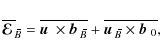
We may split the mean
electromotive force
.
We may split the mean
electromotive force
![]() likewise
and get
likewise
and get
Note that we do not restrict
![]() and
and
![]() ,
and
therefore also not
,
and
therefore also not
![]() ,
to a certain order in
,
to a certain order in
![]() .
.
In the present section we assume that the background turbulence is
purely hydrodynamic, that is,
![]() and hence
and hence
![]() .
This is possible if there is neither an external electromotive force
in the induction equation nor a small-scale dynamo. Thus,
the magnetic fluctuations
.
This is possible if there is neither an external electromotive force
in the induction equation nor a small-scale dynamo. Thus,
the magnetic fluctuations
![]() are entirely a
consequence of the interaction of the velocity fluctuations
are entirely a
consequence of the interaction of the velocity fluctuations
![]() with the mean field
with the mean field
![]() .
.
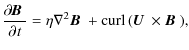
In a homogeneous medium, the induction equations for the total, mean and fluctuating magnetic fields read
with
![]() .
The solution of the linear Eq. (5) for the fluctuations
.
The solution of the linear Eq. (5) for the fluctuations
![]() ,
considered
as a functional of
,
considered
as a functional of
![]() ,
,
![]() and
and
![]() ,
is linear
and homogeneous in the latter and the same is true for
,
is linear
and homogeneous in the latter and the same is true for
If the velocity is influenced by the mean field, that is, if
The major task of mean-field theory consists now just in establishing
the linear and homogeneous functional relating
![]() to
to
![]() .
Making the ansatz
.
Making the ansatz
with
Is the result affected by the geometry of the test fields?
An ansatz like Eq. (7) is in general not exhaustive, but
restricted in its validity to a certain class of mean fields, here
strictly speaking to stationary fields which change at most linearly
in space. Consequently, the geometry of the test fields is without
relevance just as long as they are taken from the class for which
the
![]() ansatz is valid, but not for other choices.
ansatz is valid, but not for other choices.
For many applications it will be useful to generalize the test-field method
such that all employed test fields are harmonic functions of position, defined by one and the same
wavevector
![]() .
The turbulent transport coefficients can then be obtained as functions of
.
The turbulent transport coefficients can then be obtained as functions of
![]() and have to be identified with the Fourier transforms of integral kernels which define
the in general non-local relationship between
and have to be identified with the Fourier transforms of integral kernels which define
the in general non-local relationship between
![]() and
and
![]() (Brandenburg et al. 2008a).
Quite analogously,
the in general also non-instantaneous relationship between these quantities can
be recovered by using harmonic functions of time for the test fields.
The coefficients, then depending on the angular frequency
(Brandenburg et al. 2008a).
Quite analogously,
the in general also non-instantaneous relationship between these quantities can
be recovered by using harmonic functions of time for the test fields.
The coefficients, then depending on the angular frequency ![]() ,
represent again Fourier transforms
of the corresponding integral kernels
(Hubbard & Brandenburg 2009).
,
represent again Fourier transforms
of the corresponding integral kernels
(Hubbard & Brandenburg 2009).
If
![]() and
and
![]() are taken from a series of main runs with a dynamically
effective mean field of, say,
fixed geometry, but from run to run differing
strength
are taken from a series of main runs with a dynamically
effective mean field of, say,
fixed geometry, but from run to run differing
strength
![]() ,
,
![]() and
and
![]() can be obtained as functions of
can be obtained as functions of
![]() .
Thus, it is possible to determine the quenched
dynamo coefficients basically in the same way as in the kinematic
case, albeit at the cost of multiple numerical work.
.
Thus, it is possible to determine the quenched
dynamo coefficients basically in the same way as in the kinematic
case, albeit at the cost of multiple numerical work.
Let us now relax the above assumption on the background turbulence
and admit additionally a primary magnetic turbulence
![]() .
For the sake of simplicity we will not deal here with
.
For the sake of simplicity we will not deal here with
![]() ,
so let us assume that it vanishes.
In the representation Eq. (2) of
,
so let us assume that it vanishes.
In the representation Eq. (2) of
![]() we now combine the first and last terms using
we now combine the first and last terms using
![]() and obtain
and obtain
differing from Eq. (6) by the additional contribution,
3 A model problem
3.1 Motivation
We commence our study with a model problem
that is simpler than the complete MHD setup, but nevertheless shares with it the same mathematical
complications.
We drop the advection and pressure terms and adopt
for the diffusion operator simply the Laplacian (and a homogeneous medium).
Thus, there is no constraint on the velocity from
the continuity equation and an equation of state.
However, as in the full problem, we allow the magnetic field to exert a Lorentz
force on the fluid.
We also allow for the presence of
an imposed uniform magnetic field
![]() to enable a
determination of the
to enable a
determination of the ![]() effect
independently from the test-field method
by the imposed-field method.
effect
independently from the test-field method
by the imposed-field method.
The magnetic field is hence represented as
![]() ,
where
,
where
![]() is the vector potential of its non-uniform part.
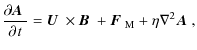
The resulting modified momentum equation for the velocity
is the vector potential of its non-uniform part.
The resulting modified momentum equation for the velocity
![]() and the (original) induction equation then read
and the (original) induction equation then read
where we have included the possibility of both kinetic and magnetic forcing
terms,
![]() and
and
![]() ,
respectively.
(In this paper we use the terms
``hydrodynamic forcing'' and ``kinetic forcing'' synonymously.)
Furthermore,
,
respectively.
(In this paper we use the terms
``hydrodynamic forcing'' and ``kinetic forcing'' synonymously.)
Furthermore, ![]() is the kinematic viscosity and
is the kinematic viscosity and ![]() the magnetic
diffusivity.
We have adopted a system of units in which
the magnetic
diffusivity.
We have adopted a system of units in which
![]() has the dimension of velocity.
Defining the current density as
has the dimension of velocity.
Defining the current density as
![]() ,
it has then the unit of inverse time.
,
it has then the unit of inverse time.
As will become clear, the major difficulty in defining a test-field method for
an MHD or purely magnetic background turbulence
is caused by bilinear (or quadratic) terms like
![]() and
and
![]() .
Hence, taking the
advective term
.
Hence, taking the
advective term
![]() into account
would not offer any new aspect, but would blur the essence of the derivation and the clear analogy
in the treatment of the former two nonlinearities.
The treatment of the advective term follows the same pattern, as is
demonstrated in Appendix A.
Given that our technique is still in its infancy, and that many underlying
issues have not been adressed yet, it is a major advantage to begin
with the simpler set of equations.
This helps significantly in clarifying the approach and in eliminating
sources of error in the numerical implementation.
into account
would not offer any new aspect, but would blur the essence of the derivation and the clear analogy
in the treatment of the former two nonlinearities.
The treatment of the advective term follows the same pattern, as is
demonstrated in Appendix A.
Given that our technique is still in its infancy, and that many underlying
issues have not been adressed yet, it is a major advantage to begin
with the simpler set of equations.
This helps significantly in clarifying the approach and in eliminating
sources of error in the numerical implementation.
In three dimensions and for
![]() ,
but with
kinetic forcing via
,
but with
kinetic forcing via
![]() ,
the system (9), (10)
is capable of reproducing
essential features of turbulent dynamos like initial exponential growth
and subsequent saturation; see, e.g., Brandenburg (2001) or
Haugen et al. (2004).
,
the system (9), (10)
is capable of reproducing
essential features of turbulent dynamos like initial exponential growth
and subsequent saturation; see, e.g., Brandenburg (2001) or
Haugen et al. (2004).
If
![]() or
or
![]() we are
no longer dealing with a dynamo problem in the strictest sense.
A discussion of dynamo processes is still
meaningful if
we are
no longer dealing with a dynamo problem in the strictest sense.
A discussion of dynamo processes is still
meaningful if
![]() and the magnetic forcing
does not give rise to a mean electromotive force
and the magnetic forcing
does not give rise to a mean electromotive force
![]() .
A possibility to accomplish this is
.
A possibility to accomplish this is
![]() together with a magnetic forcing resulting in a Beltrami field
together with a magnetic forcing resulting in a Beltrami field
![]() ,
but any choice providing an isotropic background turbulence
,
but any choice providing an isotropic background turbulence
![]() should be suited likewise.
Then, in spite of the presence of a magnetic forcing,
the mean-field induction equation is still autonomous
allowing for the solution
should be suited likewise.
Then, in spite of the presence of a magnetic forcing,
the mean-field induction equation is still autonomous
allowing for the solution
![]() .
It
depends on properties of the background turbulence like
chirality whether, e.g., the
.
It
depends on properties of the background turbulence like
chirality whether, e.g., the ![]() effect renders
this solution unstable by enabling growing solutions.
effect renders
this solution unstable by enabling growing solutions.
If we, however,
admit
![]() ,
at least in the homogeneous case the mean emf,
,
at least in the homogeneous case the mean emf,
![]() ,
is without effect and
,
is without effect and
![]() is a solution
of the mean-field induction equation which cannot grow.
Should a growing mean field nevertheless be observed, it can so legitimately
be attributed to an instability.
is a solution
of the mean-field induction equation which cannot grow.
Should a growing mean field nevertheless be observed, it can so legitimately
be attributed to an instability.
Thus, both scenarios
for
![]() have the potential to exhibit mean-field dynamos although the original induction equation is inhomogeneous
and the dynamo must not be considered as an instability of the completely non-magnetic state.
Models of this type
may well have astrophysical relevance, because
at high magnetic Reynolds numbers small-scale dynamo action is expected
to be ubiquitous.
Large-scale fields are still considered to be a consequence of an instability,
at least if there is no
have the potential to exhibit mean-field dynamos although the original induction equation is inhomogeneous
and the dynamo must not be considered as an instability of the completely non-magnetic state.
Models of this type
may well have astrophysical relevance, because
at high magnetic Reynolds numbers small-scale dynamo action is expected
to be ubiquitous.
Large-scale fields are still considered to be a consequence of an instability,
at least if there is no
![]() or any other sort of ``battery effect''.
Magnetic forcing can be regarded as a modeling tool for providing a magnetic
background turbulence when, e.g., in a DNS the conditions
for small-scale dynamo action are not afforded.
or any other sort of ``battery effect''.
Magnetic forcing can be regarded as a modeling tool for providing a magnetic
background turbulence when, e.g., in a DNS the conditions
for small-scale dynamo action are not afforded.
Quite
generally, magnetic forcing and an imposed field provide excellent means of studying
the ![]() effect, the inverse cascade of magnetic helicity, and flow properties
in the magnetically dominated regime (see, e.g., Pouquet et al. 1976;
Brandenburg et al. 2002;
Brandenburg & Käpylä 2007).
effect, the inverse cascade of magnetic helicity, and flow properties
in the magnetically dominated regime (see, e.g., Pouquet et al. 1976;
Brandenburg et al. 2002;
Brandenburg & Käpylä 2007).
3.2 Purely magnetic background turbulence
Before taking on the most general situation of both magnetic and velocity
fluctuations in the background,
it seems instructive to look
first at the case complementary to that discussed in Sect. 2.
That is, we
assume, perhaps somewhat artificially, that the background velocity
fluctuations vanish, i.e.
![]() ,
so that
,
so that
![]() .
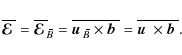
According to Eq. (2) we now find
.
According to Eq. (2) we now find
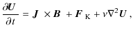
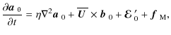
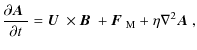
The modified momentum equation for the velocity fluctuations in a homogeneous medium reads (cf. Eq. (9))
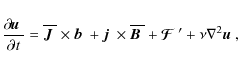
with
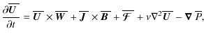
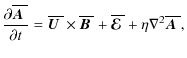
3.3 General mean-field treatment
The mean-field equations for
![]() and
and
![]() obtained by averaging
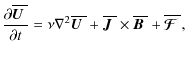
Eqs. (9) and (10) are
obtained by averaging
Eqs. (9) and (10) are
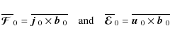
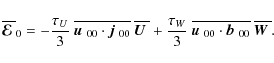
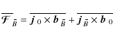
where we have assumed that the mean forcing terms vanish. From now on we extend our considerations also to the relation between the mean ponderomotive force
In the sense explained above for
In the kinematic limit
![]() and
and
![]() are expected to be non-vanishing only if
are expected to be non-vanishing only if
![]() .
An analysis in SOCA, however, would also require
.
An analysis in SOCA, however, would also require
![]() to get
a non-vanishing result; see Appendix C.
Note that
to get
a non-vanishing result; see Appendix C.
Note that
![]() allows
allows
![]() to be linear in
to be linear in
![]() ,
which would otherwise be quadratic to leading order.
Consequently, the back-reaction of the mean field onto the flow is no longer
independent of its sign.
,
which would otherwise be quadratic to leading order.
Consequently, the back-reaction of the mean field onto the flow is no longer
independent of its sign.
As
![]() is the divergence of the mean Maxwell tensor,
it has to vanish in the homogeneous case, i.e. for
homogeneous turbulence and a uniform mean field.
Hence, for Eq. (15) to be valid in physical space,
is the divergence of the mean Maxwell tensor,
it has to vanish in the homogeneous case, i.e. for
homogeneous turbulence and a uniform mean field.
Hence, for Eq. (15) to be valid in physical space,
![]() has then to vanish.
However, in Fourier space we may retain relation (15) with
has then to vanish.
However, in Fourier space we may retain relation (15) with
![]() (but not so for
(but not so for
![]() ).
On the other hand, in physical space
a description of
).
On the other hand, in physical space
a description of
![]() employing the second derivatives of
employing the second derivatives of
![]() is likely to be more appropriate, i.e.
is likely to be more appropriate, i.e.
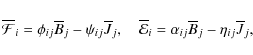
According to the expression for
would indeed be sufficient as long as there is sufficient scale separation between mean and fluctuating fields. In the following, we continue referring to
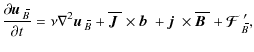
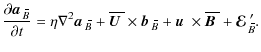
The equations for the fluctuations are obtained by subtracting Eqs. (13) from (9), and Eq. (14) from (10), what leads
to
respectively, where
Our aim is now to derive a set of formally linear equations
whose solutions, considered as
responses to a given mean field, are linear and homogeneous in the latter.
For this purpose we
make use of the split of all quantities into parts existing in the absence
of
![]() and parts vanishing with
and parts vanishing with
![]() ,
as introduced in Sect. 2.
We write
,
as introduced in Sect. 2.
We write
![]() ,
,
![]() and
and
![]() ,
as well as
,
as well as
![]() and
and
![]() ,
and assume that the forcing is independent of
,
and assume that the forcing is independent of
![]() .
Equations (17) and (18) split consequently as follows
(see Appendix D for an illustration)
.
Equations (17) and (18) split consequently as follows
(see Appendix D for an illustration)
Because of
![]() and
and
![]() ,
Eqs. (19) and (20) are completely closed. Furthermore, we have
,
Eqs. (19) and (20) are completely closed. Furthermore, we have
We can rewrite these expressions such that they become formally linear in
Now we have achieved our goal of deriving a system of formally linear equations defining the parts of the fluctuations that can be related to the mean field as response to its interaction with the given fluctuating fields
For the parts of the mean ponderomotive and electromotive forces existing already with
![]() we find
we find
|
(27) |
which could be finite due to a small-scale dynamo or magnetic forcing. Although it is hard to imagine that isotropic forcing alone is capable of enabling a non-vanishing
Here the index ``00'' refers to the fluctuating background uninfluenced by both the magnetic field and the mean flow. Beyond this specific result, too, one may expect that quite general some cross correlation of the primary turbulences is crucial. (Yoshizawa 1990; Rädler & Brandenburg 2010).
For the parts vanishing with
![]() we have
we have
We recall that for
with
3.4 Test-field method
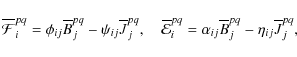
In a next step we define the actual test equations starting from Eqs. (21), (22), (25) and (26). As they are already arranged to be formally linear when deliberately ignoring the relations between
with
Correspondingly we express the mean ponderomotive and electromotive forces by the test solutions as
and stipulate that the choice within Eqs. (35) and (36) is always to correspond to the choice in Eqs. (33) and (34). As we will make use of all four possible versions we label them in a unique way by the names of the fluctuating fields of the main run that enter the expressions for
Table 1:
The four versions of the generalized test-field method as generated by combining
the different representations of
![]() and
and
![]() in Eqs. (33) and (34).
in Eqs. (33) and (34).
Now we conclude that for given
![]() ,
,
![]() ,
,
![]() ,
,
![]() and
and
![]() the test solutions
the test solutions
![]() and
and
![]() are linear and homogeneous
in the test fields
are linear and homogeneous
in the test fields
![]() and that the same holds for
and that the same holds for
![]() and
and
![]() .
Hence, the tensors
.
Hence, the tensors
![]() ,
,
![]() ,
,
![]() and
and
![]() derived from these quantities will not depend on the test fields, but
exclusively reflect properties of the given fluctuating fields and the
mean velocity.
If these are affected by a mean field in the main run the tensor
components will show a dependence on
derived from these quantities will not depend on the test fields, but
exclusively reflect properties of the given fluctuating fields and the
mean velocity.
If these are affected by a mean field in the main run the tensor
components will show a dependence on
![]() .
Thus, like in the quasi-kinematic method, quenching behavior can be identified.
We observe further that, when using the mean field from the main run as
one of the test fields, the corresponding test solutions
.
Thus, like in the quasi-kinematic method, quenching behavior can be identified.
We observe further that, when using the mean field from the main run as
one of the test fields, the corresponding test solutions
![]() and
and
![]() will coincide with
will coincide with
![]() and
and
![]() ,
respectively.
,
respectively.
Summing up, we may claim that the presented generalized test-field method in either shape satisfies certain necessary conditions for the correctness of its results. But can we be confident, that these are sufficient? An obvious complication lies in the fact that, in contrast to the quasi-kinematic method yielding the transport coefficients uniquely, we have now to deal with four different versions which need not be equivalent. Indeed we will demonstrate that the reformulation of the original problem into Eqs. (31) and (32) with Eqs. (33) and (34) introduces spurious instabilities in some applications. As we presently see no strict mathematical argument for the identity of the outcomes of all four versions, we resort to an empirical justification of our approach. This is what the rest of this paper mainly is devoted to.
Remarks:
(i) Applying the second order correlation approximation (SOCA) to the system (31), (32), that is, neglecting(ii) In the kinematic limit
(iii) For
and correspondingly
From now on we define mean fields by averaging over
two directions, here over all x and y, that is, all
mean quantities depend merely on z (if at all) and we obtain a 1D mean-field dynamo problem.
As a consequence,
![]() is constant and there are only two non-vanishing components of
is constant and there are only two non-vanishing components of
![]() ,
namely
,
namely
![]() and
and
![]() so only the evolution of
so only the evolution of
![]() and
and
![]() has to be considered.
Moreover,
has to be considered.
Moreover,
![]() is without influence on the evolution of
is without influence on the evolution of
![]() .
Hence, instead of Eqs. (15) and (7) we can write
.
Hence, instead of Eqs. (15) and (7) we can write
where the original rank-three tensors
Only the four components of either tensor with i,j=1,2 are of interest, thus
altogether 16 components need to be determined.
As one test field
![]() comprises two relevant components and yields
one
comprises two relevant components and yields
one
![]() and one
and one
![]() ,
each again with two relevant components,
we need to consider solutions of (31) through (34)
for a set of four different test fields.
,
each again with two relevant components,
we need to consider solutions of (31) through (34)
for a set of four different test fields.
Selection of test fields:
The simplest choice are uniform fields in the x and y directions, but they are only suited to determine theAll four tensors can be extracted by use of
test fields with either the xor the y component proportional to either
![]() or
or
![]() and the other vanishing
(see, e.g., Brandenburg 2005b; Brandenburg et al. 2008a,
2008b; Sur et al. 2008).
That is,
and the other vanishing
(see, e.g., Brandenburg 2005b; Brandenburg et al. 2008a,
2008b; Sur et al. 2008).
That is,
![]() is either
is either
![]() or
or
![]() ,
where the superscript
pq with p=1,2 and
,
where the superscript
pq with p=1,2 and
![]() labels the test field.
The wavenumber kz is bounded from below by
labels the test field.
The wavenumber kz is bounded from below by ![]() ,
where Lz is the extent of the computational domain in the z direction.
By varying kz, the wanted tensor components can
be determined as functions of kz. They have then no longer to be
interpreted in the usual way, but as Fourier transforms of integral kernels instead (cf. Brandenburg et al. 2008a).
In other terms, as
the harmonic test fields do not belong to the class of mean fields for which the
ansatzes (7) and (15)
are exhaustive (see Sect. 2) we must be aware that the tensors calculated in this way are ``polluted'' by contributions
from terms with higher spatial derivatives of
,
where Lz is the extent of the computational domain in the z direction.
By varying kz, the wanted tensor components can
be determined as functions of kz. They have then no longer to be
interpreted in the usual way, but as Fourier transforms of integral kernels instead (cf. Brandenburg et al. 2008a).
In other terms, as
the harmonic test fields do not belong to the class of mean fields for which the
ansatzes (7) and (15)
are exhaustive (see Sect. 2) we must be aware that the tensors calculated in this way are ``polluted'' by contributions
from terms with higher spatial derivatives of
![]() .
.
For each pair of test fields
![]() we determine
we determine ![]() unknowns
by solving the linear systems
unknowns
by solving the linear systems
q= c,s. Note that there is no coupling between the systems for p=1 and p=2. Both coefficient matrices in (39) are given by the rotation matrix
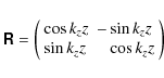
|
(40) |
(with the angle kz z) and the solutions are
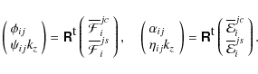
Here the superscript ``t'' indicates transposition.
3.5 Forcing functions, computational domain, and boundary conditions
For testing purposes, a common and convenient choice is the
Roberts flow forcing function,
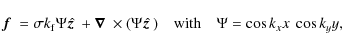
and the effective forcing wavenumber
The Roberts forcing function will be employed for kinetic as well as magnetic
forcing, so we write
![]() ,
where the
,
where the
![]() are amplitudes having
the units of acceleration and velocity squared, respectively.
Note that for
are amplitudes having
the units of acceleration and velocity squared, respectively.
Note that for ![]() ,
Eq. (42) yields a Beltrami field, i.e., it
has the property
,
Eq. (42) yields a Beltrami field, i.e., it
has the property
![]() .
Provided
.
Provided
![]() ,
the kinetic and magnetic forcings act
completely uninfluenced from each other
because a
,
the kinetic and magnetic forcings act
completely uninfluenced from each other
because a
![]() with Beltrami property exerts no Lorentz force and
with Beltrami property exerts no Lorentz force and
![]() .
Thus, a flow and a magnetic field are created that have exact Roberts geometry.
This is not the case for
.
Thus, a flow and a magnetic field are created that have exact Roberts geometry.
This is not the case for
![]() ,
because then the Beltrami property is not obeyed.
,
because then the Beltrami property is not obeyed.
The computational domain is a cuboid with quadratic base
![]() while its z extent remains adjustable and depends on the
smallest wavenumber in the z direction, kz, to be considered.
However, as the Roberts forcing function is not z dependent,
the runs from which only
while its z extent remains adjustable and depends on the
smallest wavenumber in the z direction, kz, to be considered.
However, as the Roberts forcing function is not z dependent,
the runs from which only
![]() is extracted were carried out in 2D with
kz=0.
In all cases we assume periodic boundary conditions in all directions.
is extracted were carried out in 2D with
kz=0.
In all cases we assume periodic boundary conditions in all directions.
The results presented below were obtained using
revision r13439 of the
P ENCIL C ODE![]() ,
which is a modular high-order code (sixth order in space and third-order
in time) for solving a large range of different partial differential
equations.
,
which is a modular high-order code (sixth order in space and third-order
in time) for solving a large range of different partial differential
equations.
3.6 Control parameters and non-dimensionalization
In cases with an imposed magnetic field, we set
![]() .
Along with B0,
the forcing amplitudes
.
Along with B0,
the forcing amplitudes
![]() are the most relevant control parameters.
The only remaining one is the magnetic Prandtl number,
are the most relevant control parameters.
The only remaining one is the magnetic Prandtl number,
![]() .
If not otherwise specified it is set to unity, i.e.
.
If not otherwise specified it is set to unity, i.e. ![]() .
.
It is convenient to measure length in units of the inverse minimal wavenumber k1,
time in units of
![]() ,
velocity in units of
,
velocity in units of ![]() ,
just as the magnetic field.
The forcing amplitudes
,
just as the magnetic field.
The forcing amplitudes
![]() are given in units of
are given in units of
![]() and
and
![]() ,
respectively.
Results will also be presented in dimensionless form:
,
respectively.
Results will also be presented in dimensionless form:
![]() and
and ![]() in units of
in units of ![]() ,
,
![]() in units of
in units of ![]() ,
and
,
and ![]() in units of
in units of
![]() ,
if not declared otherwise.
Dimensionless quantities are denoted by a tilde throughout.
,
if not declared otherwise.
Dimensionless quantities are denoted by a tilde throughout.
The intensities of the actual and background
turbulences are readily measured by the
magnetic Reynolds
and Lundquist numbers,
| (43) |
where
4 Results
An important criterion for the correctness of the generalized test-field methods is the agreement of their results with those of the imposed-field method which is, of course, only applicable if the actual mean field in the main run is uniform. In most cases we checked for this criterion, the being restricted to kz=0 in the test fields. On the other hand, in many cases with vanishingDue to the properties of the Roberts forcing we have
![]() throughout.
For this reason, and because in the
main runs no other mean fields than the uniform occurred, the mean flow
throughout.
For this reason, and because in the
main runs no other mean fields than the uniform occurred, the mean flow
![]() is vanishing too.
is vanishing too.
4.1 Limit of vanishing mean magnetic field
In this section we assume that the mean field is absent or
weak enough so as not to affect
the fluctuating fields markedly, that is,
![]() ,
,
![]() .
In particular, it can then not render the transport coefficients anisotropic.
Therefore, we denote by
.
In particular, it can then not render the transport coefficients anisotropic.
Therefore, we denote by ![]() and
and
![]() simply the average
of the first two diagonal
components of
simply the average
of the first two diagonal
components of
![]() and
and
![]() ,
i.e.
,
i.e.
![]() and
and
![]() ,
respectively.
If not specified otherwise we set
,
respectively.
If not specified otherwise we set
![]() or zero.
or zero.
4.1.1 Purely hydrodynamic forcing
In order to make contact with known results, we consider first the case of the hydrodynamically driven Roberts flow. In two dimensions, no small-scale dynamo is possible, hence![\begin{displaymath}\alpha/\alpha_{\rm0K}=\mbox{\rm Re}_{\rm M}/[1+(k_z/k_{\rm f})^2],\quad \alpha_{\rm0K}=-u_{\rm rms}/2,
\end{displaymath}](/articles/aa/full_html/2010/12/aa14700-10/img255.png)
where kz is the wavenumber of the harmonic test fields. The minus sign in
Making use of the quasi-kinematic method,
as well as of all four versions of the generalized method,
we calculated ![]() for
for
![]() ,
kz=0 (2D case) and values of
,
kz=0 (2D case) and values of
![]() ranging from 0.01 to 100with a ratio of 10, where
ranging from 0.01 to 100with a ratio of 10, where
![]() grows then from 0.005 to 50.
Figure 1
shows
grows then from 0.005 to 50.
Figure 1
shows
![]() versus
versus
![]() (solid line).
Here the data points for all methods are indistinguishable and agree also
with those of the imposed-field method.
(solid line).
Here the data points for all methods are indistinguishable and agree also
with those of the imposed-field method.
![\begin{figure}
\par\includegraphics[width=9cm,clip]{14700fig1}
\end{figure}](/articles/aa/full_html/2010/12/aa14700-10/img262.png)
|
Figure 1:
|
| Open with DEXTER | |
Agreement with the SOCA result Eq. (44) (dotted line) exists
for
![]() .
For
.
For
![]() ,
SOCA is not applicable, because dropping the
,
SOCA is not applicable, because dropping the
![]() term
in (32) is then no longer justified.
The SOCA values are nevertheless numerically reproducible
by the test-field methods when ignoring
the
term
in (32) is then no longer justified.
The SOCA values are nevertheless numerically reproducible
by the test-field methods when ignoring
the
![]() and
and
![]() terms in Eqs. (31) and (32);
see the diamond-shaped data points in Fig. 1.
terms in Eqs. (31) and (32);
see the diamond-shaped data points in Fig. 1.
Corrections to the result (44) with the
![]() term retained
were computed analytically by Rädler et al. (2002a,b).
The corresponding values are again well reproduced by all flavors
of the generalized test-field method
as well as by the imposed-field method.
term retained
were computed analytically by Rädler et al. (2002a,b).
The corresponding values are again well reproduced by all flavors
of the generalized test-field method
as well as by the imposed-field method.
In the first line of Table 2, we repeat the ![]() result for
result for
![]() and added that for test fields with the wavenumber kz=1,
from where we also come to know the turbulent diffusivity
and added that for test fields with the wavenumber kz=1,
from where we also come to know the turbulent diffusivity
![]() .
Note the difference between the
values for kz=1 and kz=0, which is
roughly given by a factor 3/2 for kz=1 and
.
Note the difference between the
values for kz=1 and kz=0, which is
roughly given by a factor 3/2 for kz=1 and
![]() ;
see Eq. (44).
Additionally, the results of the quasi-kinematic method for kz=1,
;
see Eq. (44).
Additionally, the results of the quasi-kinematic method for kz=1,
![]() and
and
![]() ,
are shown.
As expected, they coincide completely with
,
are shown.
As expected, they coincide completely with ![]() and
and
![]() .
.
4.1.2 Purely magnetic forcing
Next we consider the case of purely magnetic Roberts forcing, i.e.![\begin{displaymath}\alpha/\alpha_{\rm0M}= (\mbox{\rm Lu}/\mbox{\rm Pr}_{\rm M})/[1+(k_z/k_{\rm f})^2],\quad \alpha_{\rm0M}=3b_{\rm rms}/4
\end{displaymath}](/articles/aa/full_html/2010/12/aa14700-10/img276.png)
(for the derivation see Appendix E). It turns out that the sign of
![\begin{figure}
\par\includegraphics[width=9cm,clip]{14700fig2}\end{figure}](/articles/aa/full_html/2010/12/aa14700-10/img281.png)
|
Figure 2:
|
| Open with DEXTER | |
Table 2:
Dependence of
![]() and
and
![]() from
the generalized method
on
from
the generalized method
on
![]() for
for
![]() and
and
![]() together with the kinetic contribution
together with the kinetic contribution
![]() and the results from
the quasi-kinematic method (
and the results from
the quasi-kinematic method (
![]() and
and
![]() ).
).
4.2.3 Hydromagnetic forcing
In analogy to Figs. 5 and 7 we show in Fig. 8 the constituents of![\begin{figure}
\par\includegraphics[width=9cm,clip]{14700fig8}
\end{figure}](/articles/aa/full_html/2010/12/aa14700-10/img365.png)
|
Figure 8:
|
| Open with DEXTER | |
It can be observed that
![]() at first dominates over
at first dominates over
![]() ,
but at
,
but at
![]() their relation reverses. Remarkably, the ratio of their
moduli reaches, for high values of
their relation reverses. Remarkably, the ratio of their
moduli reaches, for high values of
![]() ,
just the inverse of that
for low values.
The strong quenching of
,
just the inverse of that
for low values.
The strong quenching of
![]() is now a consequence of
is now a consequence of
![]() approaching
approaching
![]() .
In complete agreement with the former two cases with pure forcings,
.
In complete agreement with the former two cases with pure forcings,
![]() is proportional to
is proportional to
![]() for strong fields.
However, we see a deviating behavior of
for strong fields.
However, we see a deviating behavior of
![]() as it is no longer following a power law.
as it is no longer following a power law.
Given that the ![]() effect can be sensitive to the value of
effect can be sensitive to the value of
![]() ,
we study
,
we study
![]() and
and
![]() as functions of
as functions of
![]() ,
keeping
,
keeping
![]() and
and
![]() fixed.
The result is shown in Fig. 9.
fixed.
The result is shown in Fig. 9.
![\begin{figure}
\par\includegraphics[width=9cm,clip]{14700fig9}
\end{figure}](/articles/aa/full_html/2010/12/aa14700-10/img373.png)
|
Figure 9:
Dependence of
|
| Open with DEXTER | |
4.3 Convergence
In most of the cases the four different versions of the generalized method
(see Table 1)
give quite similar results.
For purely hydrodynamic and purely magnetic forcing
there is agreement to all significant digits.
This is not quite so perfect with hydromagnetic forcing, i.e.
![]() ,
,
![]() .
In general, however, agreement is improved by increasing the numerical resolution.
.
In general, however, agreement is improved by increasing the numerical resolution.
![\begin{figure}
\par\includegraphics[width=9cm,clip]{14700fig10}\vspace{3mm}
\end{figure}](/articles/aa/full_html/2010/12/aa14700-10/img380.png)
|
Figure 10:
Convergence of
|
| Open with DEXTER | |
Yet another complication arises when ![]() ,
because then some of
the versions are found to display exponentially growing test
solutions; see Fig. 10.
This may not be surprising, because each version corresponds to a
different linear inhomogeneous
system of equations, and there is no guarantee
that each of them has only stable solutions.
The actual occurrence of instabilities depends however
on intricate properties of the fluctuating fields
from the main run,
,
because then some of
the versions are found to display exponentially growing test
solutions; see Fig. 10.
This may not be surprising, because each version corresponds to a
different linear inhomogeneous
system of equations, and there is no guarantee
that each of them has only stable solutions.
The actual occurrence of instabilities depends however
on intricate properties of the fluctuating fields
from the main run,
![]() and
and
![]() .
We suppose that, if one could remove the unstable eigenvalues of the homogeneous part of the system (31)-(34) from its spectrum, the solution of the inhomogeneous system would indeed be the correct one.
.
We suppose that, if one could remove the unstable eigenvalues of the homogeneous part of the system (31)-(34) from its spectrum, the solution of the inhomogeneous system would indeed be the correct one.
5 Discussion
The main purpose of the developed method consists in handling situations
in which hydrodynamic and magnetic fluctuations coexist in the background.
The quasi-kinematic method can only afford those constituents of the
mean-field coefficients that are related solely to the hydrodynamic
background
![]() ,
but the new method is capable of delivering, in
addition, those related to the magnetic background
,
but the new method is capable of delivering, in
addition, those related to the magnetic background
![]() .
Moreover, it is able to detect
mean-field effects that depend on cross correlations of
.
Moreover, it is able to detect
mean-field effects that depend on cross correlations of
![]() and
and
![]() .
We have demonstrated this with the two fluctuations being
forced externally to have
the same Roberts-like geometry. With respect to
.
We have demonstrated this with the two fluctuations being
forced externally to have
the same Roberts-like geometry. With respect to ![]() we observe a ``magneto-kinetic'' part being, to leading order, quadratic
in the magnetic Reynolds and Lundquist numbers.
It is capable of reducing
the total
we observe a ``magneto-kinetic'' part being, to leading order, quadratic
in the magnetic Reynolds and Lundquist numbers.
It is capable of reducing
the total ![]() significantly in comparison
with the sum of the
significantly in comparison
with the sum of the ![]() values resulting from purely hydrodynamic andpurely magnetic backgrounds.
In contrast, the tensors
values resulting from purely hydrodynamic andpurely magnetic backgrounds.
In contrast, the tensors
![]() and
and
![]() which give rise
to the occurrence of mean forces proportional to
which give rise
to the occurrence of mean forces proportional to
![]() and
and
![]() are,
to leading order, bilinear in
are,
to leading order, bilinear in
![]() and
and
![]() .
.
In nature, however,
external electromotive forces imprinting finite cross-correlations of
![]() and
and
![]() are rarely found.
Therefore the question regarding the
astrophysical relevance of these effects has to be posed.
Given the high values of
are rarely found.
Therefore the question regarding the
astrophysical relevance of these effects has to be posed.
Given the high values of
![]() in practically all cosmic bodies,
small-scale dynamos are supposed to be ubiquitous and do indeed provide
hydromagnetic background turbulence.
But is it realistic to expect non-vanishing cross-correlations
under these circumstances?
in practically all cosmic bodies,
small-scale dynamos are supposed to be ubiquitous and do indeed provide
hydromagnetic background turbulence.
But is it realistic to expect non-vanishing cross-correlations
under these circumstances?
Let us consider a number of similar, yet not completely identical
turbulence cells arranged in a more or less regular pattern.
As dynamo fields are solutions of the homogeneous induction
equation and the Lorentz force is quadratic in
![]() ,
bilinear cross-correlations,
,
bilinear cross-correlations,
![]() ,
obtained by averaging over
single cells can be expected to change their sign
randomly from cell to cell provided
the cellular dynamos have evolved independently from each other.
Consequently, the average over many cells would approach zero and the
,
obtained by averaging over
single cells can be expected to change their sign
randomly from cell to cell provided
the cellular dynamos have evolved independently from each other.
Consequently, the average over many cells would approach zero and the
![]() and
and
![]() effects would not occur.
In contrast, cross-correlations that are even functions of the components
of
effects would not occur.
In contrast, cross-correlations that are even functions of the components
of
![]() and their derivatives, were not rendered zero due to
random polarity changes in the small-scale
dynamo fields (e.g. the magneto-kinetic
and their derivatives, were not rendered zero due to
random polarity changes in the small-scale
dynamo fields (e.g. the magneto-kinetic ![]() ).
).
However, the assumption of independently acting cellular dynamos can be put in question when the whole process beginning with the onset of the turbulence-creating instability (e.g. convection) is taken into account. During its early stages, i.e. for small magnetic Reynolds numbers, the flow is at first unable to allow for any dynamo action, but with growing amplitude a large-scale dynamo can be excited first to create a field that is coherent over many turbulence cells. With further growth of its amplitude the (hydrodynamic) turbulence eventually enters a stage in which small-scale dynamo action becomes possible. The seed fields for these dynamos are now prevailingly determined by the already existing mean field and due to its spatial coherence the polarity of the small-scale field is not settling independently from cell to cell, thus potentially allowing for non-vanishing cross-correlations. Moreover, instead of employing the idea of a pre-existing large-scale dynamo one may claim that, given the smallness of the turbulence cells compared to the scale of the surroundings of the cosmic object, there is always a large-scale field, e.g. the galactic one, that is coherent across a large number of turbulence cells.
But even if one wants to abstain from employing the influence of a
pre-existing mean field it has to be considered that neighboring cells
are never exactly equal. Thus, in the course of the growing amplitude
of the hydrodynamic background, in some of them the small-scale dynamo
will start working first, hence setting the seed field for
its immediate neighbors.
It is well conceivable that a certain sign of, say, the cross-correlation,
![]() ,
established in one of the early starting cells
``cascades'' to more and more distant neighbors until this process
is limited by the cascades originating from other early starting cells.
Consequently, we arrive at a
situation similar to the one discussed before, yet with less extended
regions of coinciding signs of the correlation.
,
established in one of the early starting cells
``cascades'' to more and more distant neighbors until this process
is limited by the cascades originating from other early starting cells.
Consequently, we arrive at a
situation similar to the one discussed before, yet with less extended
regions of coinciding signs of the correlation.
In summary, cross-correlations and the mean-field effects connected to them
cannot be ruled out a priori.
Direct numerical simulations of
the scenarios discussed above should be performed in order to clarify the significance
of these effects.
This is equally valid for the effects due to cross-correlations
resulting in
![]() ;
see Eq. (28).
;
see Eq. (28).
In a recent paper, Courvoisier et al. (2010) discuss the range of applicability of the quasi-kinematic test-field method.
Their model consists of the equations of incompressible magneto-hydrodynamics with purely hydrodynamic forcing.
However, by imposing an additional uniform magnetic field
![]() together with the forced fluctuating velocity
a fluctuating magnetic field arises. It must be stressed that, following the line of their argument, these
fluctuations have to be considered as part of the background
together with the forced fluctuating velocity
a fluctuating magnetic field arises. It must be stressed that, following the line of their argument, these
fluctuations have to be considered as part of the background
![]() ,
that is,
they belong to
those fluctuations that occur in the absence of the mean field.
This follows from the fact that, when defining transport coefficients such
as
,
that is,
they belong to
those fluctuations that occur in the absence of the mean field.
This follows from the fact that, when defining transport coefficients such
as
![]() ,
the field
,
the field
![]() is not regarded as part
of the mean field
is not regarded as part
of the mean field
![]() ,
in contrast to our treatment;
see their Sect. 2b.
For simplicity they consider only the kinematic case and restrict the analysis to mean fields
,
in contrast to our treatment;
see their Sect. 2b.
For simplicity they consider only the kinematic case and restrict the analysis to mean fields ![]()
![]() with
with
![]() .
In their main conclusion, drawn under these conditions, they state that
the quasi-kinematic test-field method, which considers only the
magnetic response to a mean magnetic field, must fail for
.
In their main conclusion, drawn under these conditions, they state that
the quasi-kinematic test-field method, which considers only the
magnetic response to a mean magnetic field, must fail for
![]() ,
that is
,
that is
![]() .
We fully agree in this respect, but should point out that the quasi-kinematic
method was not claimed to be applicable in that case; see Brandenburg et al. (2008c, Sect. 3)
giving the caveat
``As in almost all supercritical runs a small-scale dynamo is operative,
our results which are derived under the assumption of its influence being negligible
may contain a systematic error.''.
However, Courvoisier et al. (2010) overinterpret their finding in postulating
that already the determination of quenched coefficients such as
.
We fully agree in this respect, but should point out that the quasi-kinematic
method was not claimed to be applicable in that case; see Brandenburg et al. (2008c, Sect. 3)
giving the caveat
``As in almost all supercritical runs a small-scale dynamo is operative,
our results which are derived under the assumption of its influence being negligible
may contain a systematic error.''.
However, Courvoisier et al. (2010) overinterpret their finding in postulating
that already the determination of quenched coefficients such as
![]() for
for
![]() by means of the quasi-kinematic
method leads to wrong results.
The paper of Tilgner & Brandenburg (2008), quoted by them
in this context, is just proving evidence for the correctness of the method,
as does Brandenburg et al. (2008c).
by means of the quasi-kinematic
method leads to wrong results.
The paper of Tilgner & Brandenburg (2008), quoted by them
in this context, is just proving evidence for the correctness of the method,
as does Brandenburg et al. (2008c).
Our tensor
![]() is related to their newly introduced
mean-field coefficient
is related to their newly introduced
mean-field coefficient
![]() by
by
![]() .
Unfortunately, an attempt to reproduce their results for
.
Unfortunately, an attempt to reproduce their results for
![]() (and likewise for
(and likewise for
![]() )
is not currently
possible owing to our modified hydrodynamics.
We postpone this task to a future paper.
)
is not currently
possible owing to our modified hydrodynamics.
We postpone this task to a future paper.
6 Conclusions
Having been applied to situations with a magnetohydrodynamic background where both
![]() and
and
![]() have Roberts geometry, the proposed method has proven its potential
for determining turbulent transport coefficients.
In particular, effects connected with cross-correlations between
have Roberts geometry, the proposed method has proven its potential
for determining turbulent transport coefficients.
In particular, effects connected with cross-correlations between
![]() and
and
![]() have been
identified and were found to be in full agreement with analytical predictions as far as they are available.
No basic restrictions with respect to the magnetic Reynolds number
or the strength of the mean field,
which causes the nonlinearity of the problem, are observed so far.
As a next step, of course, the simplifications in the hydrodynamics used here have to be dropped, thus
allowing to produce more relevant results and facilitating comparison with
work already done.
have been
identified and were found to be in full agreement with analytical predictions as far as they are available.
No basic restrictions with respect to the magnetic Reynolds number
or the strength of the mean field,
which causes the nonlinearity of the problem, are observed so far.
As a next step, of course, the simplifications in the hydrodynamics used here have to be dropped, thus
allowing to produce more relevant results and facilitating comparison with
work already done.
Due to the fact that we have no strict mathematical proof for its correctness, there can be no full certainty about the general reliability of the method. An encouraging hint is given by the fact that all four flavors of the method produce often nearly identical results. Occasionally, however, some of them show unstable behavior in the test solutions. Clearly, further exploration of the method's degree of reliance is necessary by including three-dimensional and time-dependent backgrounds. Homogeneity should be abandoned and backgrounds which come closer to real turbulence such as forced turbulence or turbulent convection in a layer are to be taken into account.
Thus, the utilized approach of establishing a test-field procedure
in a situation where the governing equations are inherently nonlinear
(although by virtue of the Lorentz force only)
has proven to be promising.
This fact encourages us to develop
test-field methods for determining
turbulent transport coefficients connected with
similar nonlinearities
in the momentum equation.
An interesting target is the turbulent kinematic viscosity tensor
and especially its off-diagonal components that can give rise to a mean-field
vorticity dynamo (Elperin et al. 2007; Käpylä et al. 2009),
as well as the so-called anisotropic kinematic ![]() effect
(Frisch et al. 1987; Sulem et al. 1989;
Brandenburg & von Rekowski 2001;
Courvoisier et al. 2010) and the
effect
(Frisch et al. 1987; Sulem et al. 1989;
Brandenburg & von Rekowski 2001;
Courvoisier et al. 2010) and the ![]() effect (Rüdiger 1980, 1982).
Yet another example is given by the turbulent transport coefficients
describing effective magnetic pressure and tension forces due to the
quadratic dependence of the total Reynolds stress tensor on the mean
magnetic field (e.g., Rogachevskii & Kleeorin 2007;
Brandenburg et al. 2010).
effect (Rüdiger 1980, 1982).
Yet another example is given by the turbulent transport coefficients
describing effective magnetic pressure and tension forces due to the
quadratic dependence of the total Reynolds stress tensor on the mean
magnetic field (e.g., Rogachevskii & Kleeorin 2007;
Brandenburg et al. 2010).
We thank Kandaswamy Subramanian for insightful comments that have improved the presentation of our work. This work was supported in part by the European Research Council under the AstroDyn Research Project No. 227952 and the Swedish Research Council Grant No. 621-2007-4064.
Appendix A: Incompressibility
The equations used in this paper have the advantage of simplifying the derivation of the generalized test-field method, but the resulting flows are not realistic because the pressure and advective terms are absent. Here we drop these restrictions and derive the test equations in the incompressible case with constant density. The full momentum and induction equations take then the form
| (A.1) | |||
|
(A.2) |
where
|
(A.3) | ||
|
(A.4) |
where
where

and the equations for the
where
![]() and
and
![]() with
with
![]() ,
,
![]() ,
and
,
and
| (A.11) | |||
| (A.12) |
We can rewrite these equations such that they become formally linear in
| (A.13) | |||
| (A.14) |
It is the one which comes closest to the quasi-kinematic test-field method, because there
where
| (A.17) | |||
| (A.18) |
For the mean electromotive and ponderomotive force the ansatzes Eqs. (7)
and (15) can be employed without change.
Note, however, that the tensors
![]() and
and
![]() now contain contributions from the Reynolds
stress caused by
now contain contributions from the Reynolds
stress caused by
![]() ,
that is, eventually by
,
that is, eventually by
![]() .
.
Appendix B: Completeness of ansatzes (7) and (15)
The ansatzes Eqs. (7) and (15) are not exhaustive because higher spatial and all temporal derivatives of
![]() are omitted.
Within this limitation, however,
they provide full generality with respect to the tensorial structure of the relationship between
are omitted.
Within this limitation, however,
they provide full generality with respect to the tensorial structure of the relationship between
![]() and
and
![]() or
or
![]() .
Consequently, it is not necessary to include further terms proportional
to the mean flow and its derivatives, as the corresponding coefficients
can be covered by the already included ones.
For example, to get a contribution of the form
.
Consequently, it is not necessary to include further terms proportional
to the mean flow and its derivatives, as the corresponding coefficients
can be covered by the already included ones.
For example, to get a contribution of the form
![]() in the emf we could assume that there is a part of, e.g.,
in the emf we could assume that there is a part of, e.g.,
![]() of the form
of the form
![]() with some vector
with some vector
![]() resulting in
resulting in
![]() .
Themean velocity plays the role of a ``problem parameter'' and all
transport coefficients can of course be determined as functions of it.
.
Themean velocity plays the role of a ``problem parameter'' and all
transport coefficients can of course be determined as functions of it.
Due to the neglect of the advective term
![]() and the simplification of the viscous term in the model introduced in Sect. 3.1
there is no mean ponderomotive force
and the simplification of the viscous term in the model introduced in Sect. 3.1
there is no mean ponderomotive force
![]() in the absence of the mean field.
However, in proper hydrodynamics, e.g. in the form shown in Appendix A,
this quantity shows terms
proportional to derivatives of
in the absence of the mean field.
However, in proper hydrodynamics, e.g. in the form shown in Appendix A,
this quantity shows terms
proportional to derivatives of
![]() .
Then, a corresponding test method can be tailored likewise for the coefficients in Eq. (28)
which turn into tensors for a general anisotropic background.
.
Then, a corresponding test method can be tailored likewise for the coefficients in Eq. (28)
which turn into tensors for a general anisotropic background.
Appendix C: Derivation of
 ,
,

Start with the stationary induction equation in SOCA
|
(C.1) |
Assume
![\begin{displaymath}{\mbox{$\vec{b}$ } {}_{\hspace*{-1.1pt}\,\hspace{.3mm}\overli...
...- {\rm i} k_z ~u_{0z}\overline{\mbox{\boldmath$B$ }}{}\right].
\end{displaymath}](/articles/aa/full_html/2010/12/aa14700-10/img439.png)
For the calculation of the mean force
we need further
|
|
= | (C.2) | |
| = | (C.3) |
Consequently,
| |
= | ||
| = | |||
and with
| |
= | 
|
|
|
|||
![$\displaystyle \phantom{= }+k_z^2 \big(~ \overline{u_{0z}b_{0z}} ~\overline{B}_i - \delta_{i3} \overline{u_{0z} b_{0l}}~\overline{B}_l\big)\bigg] .$](/articles/aa/full_html/2010/12/aa14700-10/img456.png)
|
The tensors are hence
| |
= | 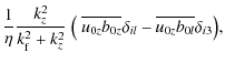
|
|
| = | 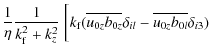
|
||
![$\displaystyle \phantom{=} + \epsilon_{lj3}\left (~ \overline{b_{0z} \frac{\part...
... {}_0}}{\partial\hspace*{.06em} {x_j}}} \delta_{i3}\right) \bigg], \quad l\ne 3$](/articles/aa/full_html/2010/12/aa14700-10/img462.png)
|
|||
| = |
For
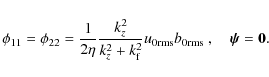
|
All other
If, however, for the Roberts geometry
![]() ,
the field
,
the field
![]() has indeed yet the property
has indeed yet the property
![]() ,
but is no longer of Beltrami type.
Instead, we have
,
but is no longer of Beltrami type.
Instead, we have
![\begin{displaymath}{\rm curl} \, {}\mbox{\boldmath$f$ } {}= \sigma k_{\rm f}\lef...
...}{\sigma^2}-1\right) f_z \hat{\mbox{\boldmath$z$ }} {}\right].
\end{displaymath}](/articles/aa/full_html/2010/12/aa14700-10/img475.png)
The tensor
| |
= | 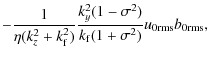
|
|
| = | 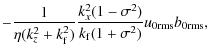
|
||
| = |
Appendix D: Illustration of extracting a linear evolution equation from a nonlinear one
To illustrate the procedure of extracting a linear evolution equation
from a nonlinear problem, let us consider a simple quadratic ordinary
differential equation, y'=y2, where a prime denotes
here differentiation.
We split y into two parts,
![]() ,
so we have
,
so we have
In the last two terms we can replace
where the last equation is linear in
Note, that the system (D.2) is exactly equivalent to (D.1), i.e. no approximation has been made.
Appendix E: Derivation of Eq. (45)
Consider the stationary version of (21) with
![]() dropped (i.e. SOCA)
dropped (i.e. SOCA)
Assume a uniform

and further
that is,
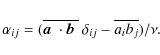
Isotropy results in
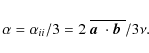
For
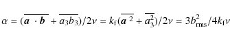
and with
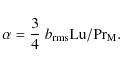
Adopt now
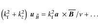
and comparison with (E.2) reveals that (E.3) has only to be modified by the factor
Appendix F: Derivation of
 in fourth order approximation
We employ the iterative procedure
described, e.g., in Rädler & Rheinhardt (2007)
to obtain those contributions to
| |
= | ||
| = |
where in the stationary case
and
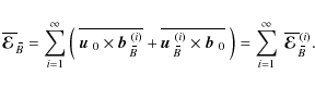
In the following we assume
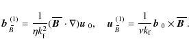
From here on we switch to dimensionless quantities and set
![\begin{eqnarray*}&&\mbox{$\vec{b}$ } {}_{\hspace*{-1.1pt}\,\hspace{.3mm}\overlin...
... 2x+2), \sin 2y\sin 2x, \sqrt{2}\sin 2y(\cos 2x+3)\right] \Big).
\end{eqnarray*}](/articles/aa/full_html/2010/12/aa14700-10/img522.png)
For
| |
= | ![$\displaystyle \frac{u_{0{\mathrm{rms}}} b_{0{\mathrm{rms}}}^2}{32}[ \sin x \sin y, \cos x \cos y, -4\sqrt{2} \sin x \cos y ]$](/articles/aa/full_html/2010/12/aa14700-10/img526.png)
|
|
| = | ![$\displaystyle \frac{u_{0{\mathrm{rms}}}^2 b_{0{\mathrm{rms}}}}{16}[ 0, \cos x \cos y, -\frac{\sqrt{2}}{2} \sin x \cos y ] + \ldots .$](/articles/aa/full_html/2010/12/aa14700-10/img529.png)
|
Finally,
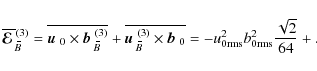
i.e.
Note, that the contributions omitted in
References
- Beck, R., Poezd, A. D., Shukurov, A., & Sokoloff, D. D. 1994, A&A, 289, 94 [NASA ADS] [Google Scholar]
- Beck, R., Brandenburg, A., Moss, D., Shukurov, A., & Sokoloff, D. 1996, ARA&A, 34, 155 [NASA ADS] [CrossRef] [Google Scholar]
- Brandenburg, A. 2001, ApJ, 550, 824 [NASA ADS] [CrossRef] [Google Scholar]
- Brandenburg, A. 2005a, ApJ, 625, 539 [Google Scholar]
- Brandenburg, A. 2005b, Astron. Nachr., 326, 787 [NASA ADS] [CrossRef] [Google Scholar]
- Brandenburg, A., & Käpylä, P. J. 2007, New J. Phys., 9, 305, 1 [Google Scholar]
- Brandenburg, A., & Subramanian, K. 2005, Phys. Rep. 417, 1 [Google Scholar]
- Brandenburg, A., & von Rekowski, B. 2001, A&A, 379, 1153 [NASA ADS] [CrossRef] [EDP Sciences] [Google Scholar]
- Brandenburg, A., Dobler, W., & Subramanian, K. 2002, Astron. Nachr., 323, 99 [Google Scholar]
- Brandenburg, A., Rädler, K.-H., & Schrinner, M. 2008a, A&A, 482, 739 [NASA ADS] [CrossRef] [EDP Sciences] [Google Scholar]
- Brandenburg, A., Rädler, K.-H., Rheinhardt, M., & Käpylä, P. J. 2008b, ApJ, 676, 740 [NASA ADS] [CrossRef] [Google Scholar]
- Brandenburg, A., Rädler, K.-H., Rheinhardt, M., & Subramanian, K. 2008c, ApJ, 687, L49 [NASA ADS] [CrossRef] [Google Scholar]
- Brandenburg, A., Kleeorin, N., & Rogachevskii, I. 2010, Astron. Nachr., 331, 5 [NASA ADS] [CrossRef] [Google Scholar]
- Cattaneo, F. 1999, ApJ, 515, L39 [NASA ADS] [CrossRef] [Google Scholar]
- Cho, J., & Vishniac, E. 2000, ApJ, 538, 217 [NASA ADS] [CrossRef] [Google Scholar]
- Courvoisier, A., Hughes, D. W., & Proctor, M. R. E. 2010, Proc. Roy. Soc. Lond., 466, 583 [Google Scholar]
- Elperin, T., Golubev, I., Kleeorin, N., & Rogachevskii, I. 2007, Phys. Rev. E, 76, 066310 [NASA ADS] [CrossRef] [Google Scholar]
- Emonet, T., & Cattaneo, F. 2001, ApJ, 560, L197 [NASA ADS] [CrossRef] [Google Scholar]
- Field, G. B., Blackman, E. G., & Chou H. 1999, ApJ, 513, 638 [NASA ADS] [CrossRef] [Google Scholar]
- Frisch, U., She, Z. S., & Sulem, P. L. Phys. D, 198728382 [Google Scholar]
- Haugen, N. E. L., Brandenburg, A., & Dobler, W. 2003, ApJ, 597, L141 [NASA ADS] [CrossRef] [Google Scholar]
- Haugen, N. E. L., Brandenburg, A., & Dobler, W. 2004, Phys. Rev. E, 70, 016308 [NASA ADS] [CrossRef] [Google Scholar]
- Hubbard, A., & Brandenburg, A. 2009, ApJ, 706, 712 [NASA ADS] [CrossRef] [Google Scholar]
- Käpylä, P. J., Korpi, M. J., & Brandenburg, A. 2008, A&A, 491, 353 [NASA ADS] [CrossRef] [EDP Sciences] [Google Scholar]
- Käpylä, P. J., Mitra, D., & Brandenburg, A. 2009, Phys. Rev. E, 79, 016302 [NASA ADS] [CrossRef] [Google Scholar]
- Käpylä, P. J., Korpi, M. J., & Brandenburg, A. 2010, MNRAS, 402, 1458 [NASA ADS] [CrossRef] [Google Scholar]
- Kazantsev, A. P. 1968, Sov. Phys. JETP, 26, 1031 [Google Scholar]
- Krause, F., & Rädler, K.-H. 1980, Mean-field magnetohydrodynamics and dynamo theory (Oxford: Pergamon Press) [Google Scholar]
- Mitra, D., Käpylä, P. J., Tavakol, R., & Brandenburg, A. 2009, A&A, 495, 1 [NASA ADS] [CrossRef] [EDP Sciences] [Google Scholar]
- Moffatt, H. K. 1972, J. Fluid Mech., 53, 385 [Google Scholar]
- Moffatt, H. K. 1978, Magnetic field generation in electrically conducting fluids (Cambridge: Cambridge University Press) [Google Scholar]
- Parker, E. N. 1979, Cosmical magnetic fields (Oxford: Clarendon Press) [Google Scholar]
- Pouquet, A., Frisch, U., & Léorat, J. 1976, J. Fluid Mech., 77, 321 [NASA ADS] [CrossRef] [Google Scholar]
- Rädler, K.-H., & Brandenburg, A. 2010, Astron. Nachr., 331, 14 [NASA ADS] [CrossRef] [Google Scholar]
- Rädler, K.-H., & Rheinhardt, M. 2007, Geophys. Astrophys. Fluid Dyn., 101, 117 [NASA ADS] [CrossRef] [MathSciNet] [Google Scholar]
- Rädler, K.-H., Rheinhardt, M., Apstein, E., & Fuchs, H. 2002a, Magnetohydrodynamics, 38, 41 [NASA ADS] [EDP Sciences] [Google Scholar]
- Rädler, K.-H., Rheinhardt, M., Apstein, E., & Fuchs, H. 2002b, Nonl. Processes Geophys., 38, 171 [NASA ADS] [CrossRef] [Google Scholar]
- Rogachevskii, I., & Kleeorin, N. 2000, Phys. Rev. E, 61, 5202 [NASA ADS] [CrossRef] [Google Scholar]
- Rogachevskii, I., & Kleeorin, N. 2007, Phys. Rev. E, 76, 056307 [NASA ADS] [CrossRef] [Google Scholar]
- Rüdiger, G. 1974, Astron. Nachr., 295, 275 [Google Scholar]
- Rüdiger, G. 1980, Geophys. Astrophys. Fluid Dyn., 16, 239 [NASA ADS] [CrossRef] [Google Scholar]
- Rüdiger, G. 1982, Geophys. Astrophys. Fluid Dyn., 21, 1 [NASA ADS] [CrossRef] [Google Scholar]
- Schekochihin, A. A., Maron, J. L., Cowley, S. C., & McWilliams, J. C. 2002, ApJ, 576, 806 [NASA ADS] [CrossRef] [Google Scholar]
- Schekochihin, A. A., Cowley, S. C., Taylor, S. F., Maron, J. L., & McWilliams, J. C. 2004, ApJ, 612, 276 [NASA ADS] [CrossRef] [Google Scholar]
- Schrinner, M., Rädler, K.-H., Schmitt, D., Rheinhardt, M., & Christensen, U. 2005, Astron. Nachr., 326, 245 [NASA ADS] [CrossRef] [Google Scholar]
- Schrinner, M., Rädler, K.-H., Schmitt, D., Rheinhardt, M., & Christensen, U. R. 2007, Geophys. Astrophys. Fluid Dyn., 101, 81 [NASA ADS] [CrossRef] [MathSciNet] [Google Scholar]
- Solanki, S. K., Inhester, B., & Schüssler, M. 2006, Rep. Prog. Phys., 69, 563 [NASA ADS] [CrossRef] [Google Scholar]
- Sulem, P. L., She, Z. S., Scholl, H., & Frisch, U. 1989, J. Fluid Mech., 205, 341 [Google Scholar]
- Sur, S., Subramanian, K., & Brandenburg, A. 2007, MNRAS, 376, 1238 [NASA ADS] [CrossRef] [Google Scholar]
- Sur, S., Brandenburg, A., & Subramanian, K. 2008, MNRAS, 385, L15 [NASA ADS] [CrossRef] [Google Scholar]
- Tilgner, A., & Brandenburg, A. 2008, MNRAS, 391, 1477 [NASA ADS] [CrossRef] [Google Scholar]
- Vögler, A., & Schüssler, M. 2007, A&A, 465, L43 [NASA ADS] [CrossRef] [EDP Sciences] [Google Scholar]
- Yoshizawa, A. 1990, Phys. Fluids B, 2, 1589 [NASA ADS] [CrossRef] [Google Scholar]
Footnotes
- ... ODE
![[*]](/icons/foot_motif.png)
- http://pencil-code.googlecode.com
- ... SOCA
- Note that in the stationary case in addition to
 now in general
 has to be required for SOCA to be applicable.
All Tables
Table 1:
The four versions of the generalized test-field method as generated by combining
the different representations of
![]() and
and
![]() in Eqs. (33) and (34).
in Eqs. (33) and (34).
Table 2:
Dependence of
![]() and
and
![]() from
the generalized method
on
from
the generalized method
on
![]() for
for
![]() and
and
![]() together with the kinetic contribution
together with the kinetic contribution
![]() and the results from
the quasi-kinematic method (
and the results from
the quasi-kinematic method (
![]() and
and
![]() ).
).
All Figures
|
|
Figure 1:
|
| Open with DEXTER | |
| In the text | |
|
|
Figure 2:
|
| Open with DEXTER | |
| In the text | |
|
|
Figure 8:
|
| Open with DEXTER | |
| In the text | |
|
|
Figure 9:
Dependence of
|
| Open with DEXTER | |
| In the text | |
|
|
Figure 10:
Convergence of
|
| Open with DEXTER | |
| In the text | |
Copyright ESO 2010
Current usage metrics show cumulative count of Article Views (full-text article views including HTML views, PDF and ePub downloads, according to the available data) and Abstracts Views on Vision4Press platform.
Data correspond to usage on the plateform after 2015. The current usage metrics is available 48-96 hours after online publication and is updated daily on week days.
Initial download of the metrics may take a while.