![\begin{threeparttable}% latex2html id marker 4238
\caption{Kinematic results for...
....9428$\space &$0.4714$$^{1}$\,
\\ [1mm]
\hline
\end{tabular}\end{threeparttable}](/articles/aa/full_html/2010/12/aa14700-10/img282.png)
Notes. (1) With SOCA. Test-field wavenumber kz=1,
except in the third column where kz=0.
These results agree with those of the imposed-field method.
![]() and
and
![]() refer to the quasi-kinematic method.
refer to the quasi-kinematic method.
The second line of Table 2 repeats
the result for
![]() ,
again
amended by those for kz=1 and
the results of the quasi-kinematic method, which is obviously
unable to produce correct answers.
This is because
the mean electromotive force is now given by
,
again
amended by those for kz=1 and
the results of the quasi-kinematic method, which is obviously
unable to produce correct answers.
This is because
the mean electromotive force is now given by
![]() ,
which is
only taken into account in the generalized method.
Note further that
,
which is
only taken into account in the generalized method.
Note further that
![]() is positive both for hydrodynamic and
magnetic forcings.
is positive both for hydrodynamic and
magnetic forcings.
4.1.3 Hydromagnetic forcing
As already pointed out in Sect. 3.5, in the absence of a mean field,
for simultaneous kinetic and magnetic Roberts forcing
with ![]() there is a solution of Eqs. (19) and (20) consisting just of the solutions
there is a solution of Eqs. (19) and (20) consisting just of the solutions
![]() and
and
![]() of
the system
when forced purely hydrodynamically
and magnetically, respectively. Again, a bifurcation leading to another
type of solution cannot be ruled out, but was not observed.
of
the system
when forced purely hydrodynamically
and magnetically, respectively. Again, a bifurcation leading to another
type of solution cannot be ruled out, but was not observed.
In contrast to what one might suppose, however,
the decoupling of
![]() and
and
![]() lets the value of
lets the value of ![]() for hydromagnetic forcing in general not be simply additive in the values for purely hydrodynamic and purely magnetic forcings.
We denote these
by
for hydromagnetic forcing in general not be simply additive in the values for purely hydrodynamic and purely magnetic forcings.
We denote these
by
![]() and
and
![]() ,
respectively.
Beyond SOCA
,
respectively.
Beyond SOCA![]() ,
the terms
,
the terms
![]() and
and
![]() in Eqs. (21) and (22) provide couplings between
in Eqs. (21) and (22) provide couplings between
![]() and
and
![]() and give rise to an additional ``magnetokinetic'' part
of
and give rise to an additional ``magnetokinetic'' part
of ![]() ,
defined as
,
defined as
![]() .
Note that we use here lower case subscripts k, m, mk
to distinguish this split of the
.
Note that we use here lower case subscripts k, m, mk
to distinguish this split of the ![]() values from that introduced at the end of
Sect. 3.3, which applies only to the nonlinear case.
In contrast, the occurrence of
values from that introduced at the end of
Sect. 3.3, which applies only to the nonlinear case.
In contrast, the occurrence of
![]() is a purely kinematic effect.
While
is a purely kinematic effect.
While
![]() and
and
![]() are, to leading order (and hence in SOCA),
quadratic in the respective background fluctuations,
the magnetokinetic term is of leading fourth order and is
representable in schematic form as
are, to leading order (and hence in SOCA),
quadratic in the respective background fluctuations,
the magnetokinetic term is of leading fourth order and is
representable in schematic form as
![]() .
.
Lines 5 and 8 of Table 2 show cases with hydromagnetic forcing
and amplitudes adjusted such that we would have
![]() if SOCA were valid.
In either case the preceding two lines present the corresponding purely forced cases.
Lines 6 to 8 refer to the SOCA versions of the generalized methods.
It can be clearly seen that the results are additive only in the latter case. The value of
if SOCA were valid.
In either case the preceding two lines present the corresponding purely forced cases.
Lines 6 to 8 refer to the SOCA versions of the generalized methods.
It can be clearly seen that the results are additive only in the latter case. The value of
![]() as inferred from lines 3 to 5, is -0.1 resulting in a considerable reduction of
as inferred from lines 3 to 5, is -0.1 resulting in a considerable reduction of ![]() in comparison with the
additive value.
This is owing to the strong forcing amplitudes, leaving the applicability
range of SOCA far behind.
in comparison with the
additive value.
This is owing to the strong forcing amplitudes, leaving the applicability
range of SOCA far behind.
![\begin{figure}
\par\includegraphics[width=9cm]{14700fig3}
\end{figure}](/articles/aa/full_html/2010/12/aa14700-10/img297.png)
![\begin{figure}
\par\includegraphics[width=18cm]{14700fig4}
\end{figure}](/articles/aa/full_html/2010/12/aa14700-10/img299.png)
|
Figure 4:
|
Figure 3 shows
![]() for equally strong velocity and magnetic fluctuations as a function of
for equally strong velocity and magnetic fluctuations as a function of
![]() together with
together with
![]() ,
,
![]() ,
,
![]() and the resulting total value
and the resulting total value ![]() .
Note the significant difference between the naive extrapolation of SOCA,
.
Note the significant difference between the naive extrapolation of SOCA,
![]() ,
and the true
,
and the true ![]() .
In its inset the figure shows the numerical values of
.
In its inset the figure shows the numerical values of
![]() in comparison to the result of a fourth order calculation
in comparison to the result of a fourth order calculation
![]() (for the derivation see Appendix F).
Clearly, the validity range of this expression extends beyond
(for the derivation see Appendix F).
Clearly, the validity range of this expression extends beyond
![]() and hence further
than the one of SOCA.
It remains to be studied whether the magnetokinetic contribution
has a significant effect also in the more general case when
and hence further
than the one of SOCA.
It remains to be studied whether the magnetokinetic contribution
has a significant effect also in the more general case when
![]() .
If so, considering
.
If so, considering ![]() to be the sum of a kinetic and a magnetic part,
as often done in quenching considerations, may turn out to be too simplistic.
to be the sum of a kinetic and a magnetic part,
as often done in quenching considerations, may turn out to be too simplistic.
Likewise one may wonder whether closure approaches to the determination of transport coefficients supposed to be superior to SOCA can be successful at all as long as they do not take fourth order correlations into account properly.
For the tensors
 and
and
 ,
,
which turn out to
show up with simultaneous hydromagnetic and magnetic forcing
only (in addition,
As a peculiarity of the Roberts flow, ![]() vanishes
in the range of validity of SOCA
if the helicity is maximum (
vanishes
in the range of validity of SOCA
if the helicity is maximum (![]() in (42)).
For this case the
first three panels of Fig. 4 show the numerically determined
dependences
in (42)).
For this case the
first three panels of Fig. 4 show the numerically determined
dependences
![]() ,
,
![]() and
and ![]() with
different values of
u0rms=b0rms(data points, dotted lines).
The last panel shows
with
different values of
u0rms=b0rms(data points, dotted lines).
The last panel shows ![]() for
for
![]() and the same forcing amplitudes as before.
As explained above,
and the same forcing amplitudes as before.
As explained above,
![]() and
and
![]() can now no longer be forced independently from each other.
Hence, both fields cannot show exactly the geometry defined by (42) and
u0rms and
b0rmsdiverge increasingly with increasing forcing.
can now no longer be forced independently from each other.
Hence, both fields cannot show exactly the geometry defined by (42) and
u0rms and
b0rmsdiverge increasingly with increasing forcing.
As demonstrated in Appendix C,
![]() ,
,
![]() in the SOCA limit.
For comparison these functions are depicted by solid lines.
Note the clear deviations from SOCA for
in the SOCA limit.
For comparison these functions are depicted by solid lines.
Note the clear deviations from SOCA for
![]() ,
particularly in
,
particularly in ![]() .
Note also that the expression for
.
Note also that the expression for ![]() was derived under the assumption that the background has the geometry (42).
It is therefore not applicable in a strict sense. The clear disagreement with the values
of
was derived under the assumption that the background has the geometry (42).
It is therefore not applicable in a strict sense. The clear disagreement with the values
of ![]() from the test-field method
for
high values of
from the test-field method
for
high values of
![]() and
and
![]() are hence not only due to violating the
SOCA validity constraint.
are hence not only due to violating the
SOCA validity constraint.
4.2 Dependence on the mean magnetic field
We now admit dynamically effective mean fields
and hence have to deal with anisotropic fluctuating fields
![]() and
and
![]() which result in anisotropic tensors
which result in anisotropic tensors
![]() ,
,
![]() ,
,
![]() and
and
![]() .
For the chosen forcing,
.
For the chosen forcing,
![]() is the only
reason for anisotropy in the xy plane, so
is the only
reason for anisotropy in the xy plane, so
![]() has to have the form
has to have the form

with
In general, we leave in this section safe mathematical grounds and enter empirical work.
Only for vanishing magnetic background,
![]() ,
one version of the generalized method does coincide with the quasi-kinematic one
(see Sect. 3.4, Remark (iii)) and will therefore guarantee correct results.
,
one version of the generalized method does coincide with the quasi-kinematic one
(see Sect. 3.4, Remark (iii)) and will therefore guarantee correct results.
4.2.1 Purely hydrodynamic forcing
In this case we have
![]() and all flavors of the generalized method have to
yield results which coincide with those of the quasi-kinematic method.
This is valid to very high accuracy for the ju and bu
versions and somewhat less perfectly so for the bb and jb versions.
We emphasize that the presence of
and all flavors of the generalized method have to
yield results which coincide with those of the quasi-kinematic method.
This is valid to very high accuracy for the ju and bu
versions and somewhat less perfectly so for the bb and jb versions.
We emphasize that the presence of
![]() ,
being solely
responsible for the occurrence of magnetic fluctuations, does not result
in a failure of the quasi-kinematic method as one might conclude from
the model used by Courvoisier et al. (2010).
,
being solely
responsible for the occurrence of magnetic fluctuations, does not result
in a failure of the quasi-kinematic method as one might conclude from
the model used by Courvoisier et al. (2010).
Figure 5 presents
the constituents of
![]() as functions
of the imposed field in the 2D case.
We may conclude from the data
that
as functions
of the imposed field in the 2D case.
We may conclude from the data
that ![]() is negative and approximately equal to
is negative and approximately equal to
![]() .
For values of
.
For values of
![]() ,
its modulus
approaches
,
its modulus
approaches
![]() and thus gives rise to the strong quenching of the effective
and thus gives rise to the strong quenching of the effective
![]() .
Indeed,
.
Indeed,
![]() can be described by a power law with an exponent -4 for large
can be described by a power law with an exponent -4 for large
![]() .
This is at odds with analytic results predicting either
.
This is at odds with analytic results predicting either
![]() (Field et al. 1999;
Rogachevskii & Kleeorin 2000) or
(Field et al. 1999;
Rogachevskii & Kleeorin 2000) or ![]() B-3(Moffatt 1972; Rüdiger 1974).
By comparing with computations in which the non-SOCA term was neglected,
we have checked that our discrepancy with these predictions is not a consequence of SOCA
applied therein.
Sur et al. (2007) suggested that the B-2 and B-3 dependence is likely to be valid
for time-dependent and steady flows, respectively.
It should be noted, however, that their numerical values for the steady ABC flow
do actually exhibit the B-4 power law; cf. their Fig. 2.
They also found that an
B-3(Moffatt 1972; Rüdiger 1974).
By comparing with computations in which the non-SOCA term was neglected,
we have checked that our discrepancy with these predictions is not a consequence of SOCA
applied therein.
Sur et al. (2007) suggested that the B-2 and B-3 dependence is likely to be valid
for time-dependent and steady flows, respectively.
It should be noted, however, that their numerical values for the steady ABC flow
do actually exhibit the B-4 power law; cf. their Fig. 2.
They also found that an
![]() ,
defined similarly to our
,
defined similarly to our
![]() ,
increases quadratically with
,
increases quadratically with
![]() for weak fields and
declines quadratically for strong fields.
This is in agreement with our present results.
for weak fields and
declines quadratically for strong fields.
This is in agreement with our present results.
4.2.2 Purely magnetic forcing
Here, the mean electromotive force is simply
In Fig. 6 we show the rms values of the resulting
velocity and magnetic fields
as functions of the imposed field strength for
![]() ,
corresponding to
,
corresponding to
![]() if
if
![]() .
The data points can be fitted by expressions of the form
.
The data points can be fitted by expressions of the form
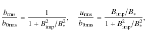
where
![\begin{figure}
\par\includegraphics[width=9cm,clip]{14700fig5}\end{figure}](/articles/aa/full_html/2010/12/aa14700-10/img328.png)
The resulting finding, as shown in Fig. 7, is completely
analogous to the one of Sect. 4.2.1, but now we see
![]() approaching
approaching
![]() with increasing
with increasing
![]() .
Hence, the idea that the quasi-kinematic method could give
reasonable results for strong mean fields has not proven true as
.
Hence, the idea that the quasi-kinematic method could give
reasonable results for strong mean fields has not proven true as
![]() is not approaching
is not approaching
![]() ,
despite the domination
of
,
despite the domination
of
![]() over
over
![]() .
Instead, the values from the quasi-kinematic method have the wrong sign and
deviate in their moduli by several orders of magnitude.
.
Instead, the values from the quasi-kinematic method have the wrong sign and
deviate in their moduli by several orders of magnitude.
![\begin{figure}
\par\includegraphics[width=9cm,clip]{14700fig6}
\end{figure}](/articles/aa/full_html/2010/12/aa14700-10/img331.png)
|
Figure 6:
Root-mean-square values
|
![\begin{figure}
\par\includegraphics[width=9cm,clip]{14700fig7}
\end{figure}](/articles/aa/full_html/2010/12/aa14700-10/img332.png)
|
|
10-2 | 1 | 101 | 102 |
|
|
|
|
|
|
|
|
|
|
|
|
|
|
|
|
|
|
|
|
|
|
|
|
|
|
|
|
|
|
Current usage metrics show cumulative count of Article Views (full-text article views including HTML views, PDF and ePub downloads, according to the available data) and Abstracts Views on Vision4Press platform.
Data correspond to usage on the plateform after 2015. The current usage metrics is available 48-96 hours after online publication and is updated daily on week days.
Initial download of the metrics may take a while.