| Issue |
A&A
Volume 528, April 2011
|
|
|---|---|---|
| Article Number | A79 | |
| Number of page(s) | 7 | |
| Section | Astrophysical processes | |
| DOI | https://doi.org/10.1051/0004-6361/201014449 | |
| Published online | 04 March 2011 | |
Stellar Mixing
IV. The angular momentum problem⋆
1 NASA, Goddard Institute for Space
Studies, New
York, NY 10025, USA
2 Department of Applied Physics and
Applied Mathematics, Columbia University, New York, NY
10027,
USA
e-mail: This email address is being protected from spambots. You need JavaScript enabled to view it.
Received: 17 March 2010
Accepted: 10 October 2010
Abstract
We present a formalism that provides the Reynolds stresses needed to solve the angular momentum equation. The traditional Reynolds stress model assumes that the only contribution comes from shear (a down-gradient flux), but this leads to an extraction of angular momentum from the interior that is far too small compared to what is required to explain the helio seismological data. An illustrative solution of the new Reynolds stress equations shows that the presence of vorticity in a stably stratified regime, such as the one in the radiative zone, contributes a new term to the angular momentum equation that has an up-gradient flux like the one provided by the IGW model (internal gravity waves). The time scale entailed by such a term may be of the same order of 107 yrs produced by the IGW model. It would be instructive to solve the new angular momentum equation together with the formalism developed in Paper III to study not only the solar angular momentum distribution vs. helio data, but also the evolution of elements such as 7Li and 4He. These results would allow a more quantitative assessment of the overall model.
The complete model yields Reynolds stresses that include differential rotation, unstable/stable stratification, double diffusion, radiative losses (arbitrary Peclet number), and meridional currents.
Key words: turbulence / diffusion / convection / hydrodynamics / methods: analytical / stars: rotation
This work is dedicated to Aura Sofia Canuto.
© ESO, 2011
1. Introduction
Helio-seismological data have presented us with an interesting new feature: solar rotation changes from differential in the convective zone CZ to uniform in the radiative, stably stratified region below the CZ. The problem has been studied for many years by many authors, and in what follows we present a brief summary of the present situation:
-
1.
3D numerical simulations by Brummel et al.(2002) and Brun & Toomre (2002) have made “promisingcontacts” with the convective zone but have not yet explained theuniform rotation in the radiative regime. The reason identified bythe authors of those studies is the limited range of physicalparameters (compared to the true solar values) allowed bynumerical simulations, e.g., the simulations are still too viscous;
-
2.
use of the angular momentum equation with Reynolds stresses with the “standard down gradient flux” for the Reynolds stresses (shear only) leads to an extraction of angular momentum from the interior that is too weak to explain the helio data. Such models yield large rotation gradients (in the stellar interiors) that are not consistent with helio data;
-
3.
several authors suggested that a different process is needed, internal gravity waves (IGW) which are characterized by an up-gradient flux (Kumar & Quataert 1997; Zahn et al. 1997; Kumar et al. 1999; Charbonnel & Talon 2005, 2007; Talon & Charbonnel 2005). The time scale required by the IGW mechanism to arrive at a solar rotational curve compatible with the helio data was estimated to be ~ 107 yrs;
-
4.
we show that, if in addition to shear generated down-gradient fluxes, one includes vorticity and stable stratification, the new Reynolds stresses contain an up-gradient term that in the radiative zone (RZ), where Ω(r) becomes close to rigid, dominates the shear down-gradient term. For small Ri corresponding to a strong shear, as expected in the CZ-RZ transition zone, the time scale can be of the same order as the one provided by the IGW mechanism.
In the next sections, we first show why the angular momentum equation employed in all previous studies is an approximation of the complete one. We then derive and show how to include vorticity and stratification, which contribute with opposite signs in the CZ and in the RZ zones where they produce an up-gradient flux in the angular momentum equation.
Finally, we show how the new Reynolds stress model includes unstable stratification, stable stratification, differential rotation, double-diffusion, arbitrary Peclet number (accounting for radiative losses), and meridional currents.
2. The solar angular momentum problem
Talon & Charbonnel (2005) have summarized the successes and failures of the “hydro-dynamically induced” processes in stellar structure studies. Here, we limit ourselves to discussing the “failures” or incompleteness of such models, the most notorious of which concerns the sun since, as Thompson et al. (2003, Sect. 7.3) have written, “calculations based on the angular momentum equation:
 (1a)predict rotation of the solar interior at a rate several times higher than the surface rate, in stark disagreement with helio data of nearly uniform rotation”. Equation (1a) is the standard equation used in all studies we have consulted (e.g., Talon & Zahn 1998; Maeder & Meynet 2001; Talon & Charbonnel 2003; Mathis et al. 2004; Palacios et al. 2003, 2006). Equation (1a) is a particular case of the general equation that can be derived from the Navier-Stokes equations for the mean velocity
  :
: 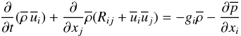 (1b)where
  are the Reynolds stresses representing the effect of turbulence on the mean flow (the total velocity field has a mean component denoted by an overbar and a fluctuating component denoted by a prime). The
  component of Eq. (1b) reads, with J = r2Ω, as
 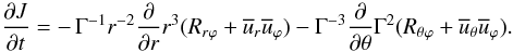 (1c)Since the equations for the meridional currents
  ,
,  , given in Sect. 6, also depend on the Reynolds stresses, we concentrate on the latter. Thus far, all models have assumed that Rij is contributed only by shear Sij, that is, they adopted the following model: Down-gradient type:
  (1d)where
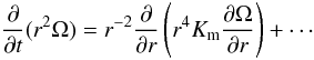
  (1e)where Km > 0 is a momentum diffusivity. Use of Eqs. (1d), (1e) in (1c) and integration over angles yield (1a). There are several problems with (1d). The first is the need to justify why only shear enters, and second is how one determines the momentum diffusivity. The first item is almost never discussed and the determination of Km is handled with heuristic models discussed in Sect. 5 of Paper II, that is, most of the attention was devoted to the determination of Km and very little, if any, to the completeness of the “shear alone” model (1d). This leads to (1a), which is not a diffusion equation, in spite of being generally referred to as such. In fact, we show that inclusion of vorticity and stratification adds to (1a) a new term that has a truly diffusive character:
  (1f)Here, N is the Brunt-Väisäla frequency
  and τ = 2K / ε (K is the eddy kinetic energy and ε its rate of dissipation) is the dynamical time scale that will be determined later. The key point is that in the CZ where x < 0, Eq. (1f) is still of the down-gradient type like (1a), but in the RZ where x > 0, Eq. (1f) becomes of the up-gradient type1:
  (1g)
This means that the generally assumed down-gradient nature of shear instabilities is incorrect at least in the context of stellar interiors where the transition from unstable to stable stratification changes the nature of the instabilities making it up-gradient. The new feature is entirely due to the combination of vorticity+buoyancy, as Eq. (1g) shows. An additional, interesting feature of (1g) is that it does not vanish for Ω = const. characterizing the radiative zone, whereas in the same regime, Eq. (1a) has a zero rhs. In conclusion, as one approaches the radiative zone, the dominant term is the non-vanishing up-gradient term (1g).
(1g)
This means that the generally assumed down-gradient nature of shear instabilities is incorrect at least in the context of stellar interiors where the transition from unstable to stable stratification changes the nature of the instabilities making it up-gradient. The new feature is entirely due to the combination of vorticity+buoyancy, as Eq. (1g) shows. An additional, interesting feature of (1g) is that it does not vanish for Ω = const. characterizing the radiative zone, whereas in the same regime, Eq. (1a) has a zero rhs. In conclusion, as one approaches the radiative zone, the dominant term is the non-vanishing up-gradient term (1g).
In the next sections, we show that shear alone giving rise to (1a) is not a justifiable approximation, and then we proceed to extend (1d) to include vorticity, buoyancy, radiative losses, double diffusion, and meridional currents.
3. Why shear alone?
Consider the first relation in Eq. (1d). It represents the first term in a Taylor expansion in the parameter τ / T where τ is the dynamical time scale while T is a typical time scale characterizing the mean flow. This can be seen by rewriting the first of (1d) as follows:  (2a)where we have employed the following relations:
  (2b)There is no physical reason why τ / T should be small, which would justify stopping at the first term (2a), and non-perturbative derivations of the Reynolds stresses (Taulbee 1992; Gatski & Speziale 1993) showed there are higher order terms in powers of τ / T. A second consideration is that (1d) requires that the principal axes of the tensor τij representing turbulence be aligned with those of Sij representing the mean flow. This is true for the case of pure strain but not for flows with a mean vorticity, which is defined as
  (2c)which is not zero even when shear is zero since shear and vorticity are two independent, orthogonal tensors, that is, when Ω → rigid body, Srϕ → 0, Vrϕ ≠ 0. For a 3D flow, in general, the measured flow distribution can only be predicted by choosing different viscosities for each stress component (Markatos 1987). In fact, a complete derivation of (1d) shows the presence of non-isotropic terms that break the “alignment assumption” and that are ultimately responsible for the extra terms discussed above. In other words, in lieu of the first of (1d), one has (Taulbee 1992; Gatski & Speziale 1993) an expression of the type
  (2d)of which the form (8h) of Paper I is the specific form after the closure constants have been determined (a ≈ 0,b = c = 1 / 10), a relation that, for completeness, we repeat here:
  (2e)The traceless tensors Σij,Zij,Bij are defined as
 where
where  is the buoyancy flux, where Eqs. (7f), in Paper I comprises both heat and μ fluxes and where
  . Thus, in going from (1d) to (2e), we have gone from
  (2i)where S, V, B stand for shear, vorticity and buoyancy. Given the incompleteness of the lhs of (2i), the failures of (1a) referred to by Thompson et al. (2003) may look less surprising, since in reality (1a) should contain shear, vorticity, and buoyancy. Other considerations are also in order. First, as we have already alluded to, one would expect the rhs of (1a) to exhibit a diffusion form while (1a) does not, though it is generally, but improperly, referred to as a “diffusion equation”. Since diffusion involves small scales, it is clear that shear, which is governed by large scales, cannot represent diffusion. Since small scales have large vorticity, it is only natural that the latter be present in (2i). Indeed, one may notice that the second of (2c) contains the angular momentum r2Ω, whereas shear, Eq. (1e), does not. Therefore, both the physical interpretation of vorticity dominated by small-scale processes (of diffusive nature) and its mathematical structure, indicate that its presence in the angular momentum equation will give rise to “diffusion”. Second, to properly describe the qualitative difference in the rotation curves in the convective and radiative regimes, it is only natural to have the buoyancy flux, which is positive in the first and negative in the second regime. The presence of B in (2i) is therefore not only natural but physically required. Third, what about the Peclet number representing radiative losses? If we recall Eq. (13j) of Paper I, it is clear that Pe is large in the CZ and small in the radiative region. This is because both the eddy velocity and the length scale are large in the CZ but small in the stably stratified radiative regime. Thus, Eq. (2i) must be extended to read as
  (2j)Finally, what about meridional currents? As shown above, they enter directly into the angular momentum Eqs. (1b), (1c) and thus we further generalize (2j) to the form
  (2k)
where M stands for meridional currents. If we succeed in constructing (2k), we would have included shear, vorticity, different regimes of both unstable (convective zone, CZ) and stable stratification (radiative regime, RZ), radiative losses, and meridional currents. While there is no guarantee that the resulting rotational curve will explain the helio data, we would have at least made sure that we have included the key processes that characterize the two regimes of interest, CZ and RZ. The RSM (Reynolds stress model) that we have presented in Paper I, is the model we employ next to compute the complete Reynolds stress Rij.
(2k)
where M stands for meridional currents. If we succeed in constructing (2k), we would have included shear, vorticity, different regimes of both unstable (convective zone, CZ) and stable stratification (radiative regime, RZ), radiative losses, and meridional currents. While there is no guarantee that the resulting rotational curve will explain the helio data, we would have at least made sure that we have included the key processes that characterize the two regimes of interest, CZ and RZ. The RSM (Reynolds stress model) that we have presented in Paper I, is the model we employ next to compute the complete Reynolds stress Rij.
4. Previous results of the RSM model
It is fair to ask whether the RSM has been previously employed in a stellar context. In answer to this question, we point to the work of Kupka and collaborators (reviewed in details in Kupka & Muthsam 2007; Kupka 2009), who studied turbulent convection using an RSM model in which the stresses and heat flux depend on time, but without rotation. Use of (2k) with rotation was made under the following conditions and with the following results. Under unstably stratified conditions, without meridional currents and using the observed rotational curve (Ulrich et al. 1988),  (3a)the model results for the Reynolds stresses
  (3b)were compared with existing solar surface measurements (Virtanen 1989; Pulkkinen et al. 1993). None of the models with
  (3c)were able to reproduce the measured surface data of (3b). In particular, the first two combinations in (3c) gave the wrong sign in both hemispheres. Only the combination
  (3d)was able to reproduce the data (Canuto et al. 1994), a conclusion that should be viewed as a useful hint when describing regimes removed from the surface. However, as already discussed, thus far all the solutions of the angular momentum equation, which yielded results in disagreement with helio data, were based on the same assumption, the first of (3c), which failed to reproduce the surface values of (3b).
5. Reynolds stresses, heat, and concentration fluxes
The specific form of the equation for the Reynolds stresses has the structure (2e), and its complete form is (see Paper I, Eq. (8h)) 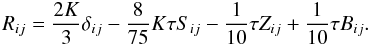 (4a)In (4a), the vorticity and buoyancy tensors were defined in Eqs. (2f) − (2h), while shear and vorticity Sij and Vij were defined in Eqs. (1e) and (2c). The density fluxes (heat and concentration fluxes) appearing in (2h) are defined as
  (4b)The heat
  and concentration fluxes
  are given by the following algebraic equations (Paper I, Eqs. (10a), (10b) and (12d), (12e)):
Heat fluxes: ![Mathematical equation: % subequation 1253 0 \begin{eqnarray} &&(\delta _{ij} +\mu _{ij} )J_j^h =\gamma _{ij} \beta _j\nonumber\\ &&\gamma _{ij} = \pi _4 \tau (R_{ij} -g\alpha _c \pi _2 \tau \lambda _i J_j^c ) \nonumber \\ && \mu _{ij} =\,\pi _4 \tau \left[S_{ij} +V_{ij} -g\tau \lambda _i (\pi _5 \alpha _T \beta _j +\pi _2 \alpha _c \overline C _{,j} )\right] .\label{eq17} \end{eqnarray}](/articles/aa/full_html/2011/04/aa14449-10/aa14449-10-eq67.png) (5a)Concentration fluxes:
(5a)Concentration fluxes: ![Mathematical equation: % subequation 1253 1 \begin{eqnarray} &&(\delta _{ij} +\eta _{ij} )J_j^c =-\,d_{ij} \overline C _{,j} \nonumber\\ && d_{ij} = \pi _1 \tau (R_{ij} +g\alpha _T \pi _2 \tau \lambda _i J_j^h ) \nonumber\\ &&\eta _{ij} =\,\pi _1 \tau \left[S_{ij} +V_{ij} -g\tau \lambda _i (\pi _2 \alpha _T \beta _j +\pi _3 \alpha _c \overline C _{,j} )\right] \label{eq18} \end{eqnarray}](/articles/aa/full_html/2011/04/aa14449-10/aa14449-10-eq68.png) (5b)\arraycolsep1.75ptwhere
(5b)\arraycolsep1.75ptwhere  (5c)The dimensionless time scales represented by the functions π′s defined in Paper I Eq. (10c), are given by:
 ![Mathematical equation: % subequation 1253 3 \begin{eqnarray} \pi _1 &=&\,\pi _1^0 \left(1+\frac{RiR_\mu }{a+R_\mu }\right)^{-1},\quad \pi _4 =\,\pi _4^0 f({\rm Pe})\left(1+\frac{Ri}{1+aR_\mu }\right)^{-1} \nonumber\\ \pi _2 &=&\pi _2^0 (1+Ri)^{-1}[1+ 2RiR_\mu (1+R_\mu ^2 )^{-1}],\, \pi _5 =\pi _5^0 g({\rm Pe}),\nonumber\\ \pi _1^0 &=&\pi _4^0 =(27Ko^3/5)^{-1/2}(1+\sigma _t^{-1} )^{-1},\nonumber \\ \pi _2^0 &=&1/3, \pi _3 =\pi _3^0 =\pi _5^0 =\sigma _t \nonumber\\ f({\rm Pe})&=&b{\rm Pe}(1+b{\rm Pe})^{-1},\nonumber\\ g({\rm Pe})&=&c{\rm Pe}(1+c{\rm Pe})^{-1}, 4\pi ^2b\!=\!5(1+\sigma _t^{-1} ), 7\pi ^2c\!=\!4\sigma _t^{-1}.\label{eq20} \end{eqnarray}](/articles/aa/full_html/2011/04/aa14449-10/aa14449-10-eq71.png) (5d)In addition, the Peclet number Pe that quantifies radiative losses is given by (Canuto & Dubovikov 1998; Paper II, Eq. (5b), with τ = 2K / ε)
(5d)In addition, the Peclet number Pe that quantifies radiative losses is given by (Canuto & Dubovikov 1998; Paper II, Eq. (5b), with τ = 2K / ε) 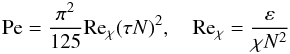 (5e)where Reχ is the Reynolds number based on the thermometric diffusivity (χis in cm2 s-1; Pr = ν / χ ≈ 10-8 is the Prandtl number). The Richardson number Ri, the density ratio Rμ, the Brunt-Väisäla frequency, and the mean shear are defined as
 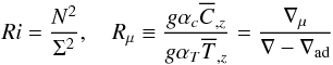 (6a)
(6a) (6b)In summary, the above formalism, which is entirely algebraic, contains the following physical ingredients:
  (6c)Once Eqs. (4a) and (5a), (5b) are solved in spherical coordinates, the resulting Reynolds stresses have the general form (2k) and can then be substituted in (1c) whose solution may then be compared with the helio data. Clearly, such a computation must be done in conjunction with a solar structure code to provide the mean variables. One can actually perform two computations, with and without double-diffusion, and compare the results, a process that would be quite instructive.
5.1. the variables K, τ
The above equations still depend on two turbulence variables represented by τ = 2Kε-1 and K, which often enter together, a product that can be written as  (7a)These are all equivalent expressions highlighting different variables; for example, the last expression is the well known 1926 Richardson law discovered fifteen years before the advent of the Kolmogorov law. In (7a) use was made of the relation ε = ℓ-1K3 / 2, where ℓ represents a typical eddy size. No matter which of the representations (7a) one chooses, the basic fact is that one must specify two independent variables, K − ε or, alternatively, K − τ. As discussed in Sect. 3 of Paper II, one must in principle solve two differential equations for the two variables K − ε given by Eqs. (II, (8a), (8b)). However, this is seldom done because of the added complexity. Instead of the equation for K, one uses its local limit corresponding to assuming production = dissipation, that is,
  (7b)where the shear and buoyancy components are given by
  (7c)
which provides the time scale τ as a function of the large-scale variables such as shear, vorticity and temperature gradients. See for example Eqs. (9d), (9e) of Paper II. The other variable ε is discussed in Sect. 3 Paper II.
(7c)
which provides the time scale τ as a function of the large-scale variables such as shear, vorticity and temperature gradients. See for example Eqs. (9d), (9e) of Paper II. The other variable ε is discussed in Sect. 3 Paper II.
6. Meridional currents
In addition to Eq. (1c) for  , for completeness we also write down the model independent general dynamic equations for the meridional currents
  :
: 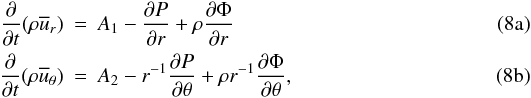 where
where 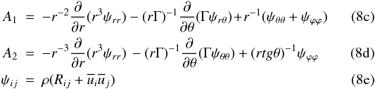 where P is the mean pressure and Φ is gravitational potential. Equations (8) show that the meridional currents depend on the Reynolds stresses as well.
7. Example: no meridional currents – no double diffusion
In Canuto & Minotti (2001), we presented the explicit solution of Eqs. (4a) and (5a) including meridional currents. The solutions represented by nested algebraic relations, were suited to a numerical treatment but not to physical considerations. Here, we present a solution of the same equations with no meridional currents and no double diffusion, a simplification that allows highlighting a new feature of the model, the existence of a counter-gradient angular momentum flux within the hydrodynamic instability framework. We begin by introducing the following dimensionless variables: 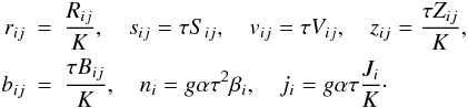 (9a)The dimensionless form of Eq. (4a) then reads
 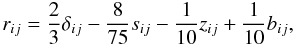 (9b)where
 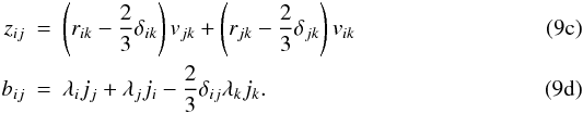 The dimensionless form of Eq. (5a) reads as
 (9e)Equations (9b) − (9e) form a system of linear, coupled, algebraic equations that may be solved using a method of symbolic algebra; additionally, we must solve the relation P = ε which, using (9a), reads as:
  (9f)For illustrative purposes, we take
  (10a)Solving (9b) − (9e), the resulting Reynolds stress and heat fluxes have the forms:
  (10b)where
  (10c)Here, Sm,h are dimensionless structure functions that depend on the parameters of the problem and that are obtained once Eq. (9b) is solved, as plotted in Fig. 2. Using the relations uϕ = rΓΩ(r,θ), ur = uθ = 0, Γ = sinθ, we further have
  (10d)with Sϕr + Vϕr = − ΓΩ, and we introduced the dimensionless variables:
  (10e)Solving (9f), one obtains the functions
  (10f)The angular momentum Eq. (1c) then becomes:
 ![Mathematical equation: \begin{equation} \label{eq43} \frac{\partial }{\partial t}(r^2\Omega ) = r^{-2}\frac{\partial }{\partial r}\left(\nu _t r^4S_{m}^{(1)} \frac{\partial \Omega }{\partial r}\right)-r^{-2}\frac{\partial }{\partial r}\left[\nu _t xS_{m}^{(2)} r^2\frac{\partial r^2\Omega }{\partial r}\right]\cdot \end{equation}](/articles/aa/full_html/2011/04/aa14449-10/aa14449-10-eq114.png) (11)The first term has the same form as in (1d), while the second term includes the contribution of vorticity and stratification x. Several comments are in order:
(11)The first term has the same form as in (1d), while the second term includes the contribution of vorticity and stratification x. Several comments are in order:
- 1.
Vorticity and buoyancy appear together in (10b), which issomething of a surprise since such a combination was not obviousin the starting Eqs. (9b) − (9e).
- 2.
Since x represents stratification, we have x < 0 in the CZ (convective zone) and x > 0 in the RZ (radiative zone).
- 3.
The first term in the rhs of (11) is independent of stratification and does not have the form of a diffusion of J = r2Ω, as we have already pointed out in the discussion after Eq. (1f). The second term in (11) is of the diffusion type, and its sign depends on whether one is in the CZ x < 0 or in the RZ zone, x > 0. There is an alternative representation of (11) with the form
![Mathematical equation: % subequation 1789 0 \begin{eqnarray} \label{eq44} \frac{\partial }{\partial t}(r^2\Omega ) &= &r^{-2}\frac{\partial }{\partial r}\left(\Gamma _{m}^{(1)} \frac{\varepsilon }{\Omega ^2}r^4\frac{\partial \Omega }{\partial r}\right)\nonumber\\[2mm] &&-r^{-2}\frac{\partial }{\partial r}\left[\Gamma _{m}^{(2)} \frac{\varepsilon }{\Omega ^2}r^2\frac{\partial r^2\Omega }{\partial r}\right], \end{eqnarray}](/articles/aa/full_html/2011/04/aa14449-10/aa14449-10-eq117.png) (12a)where we have defined the two dimensionless variables:
(12a)where we have defined the two dimensionless variables:  (12b)
(12b)
 by rewriting (12a) as
 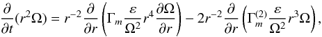 (13)where
 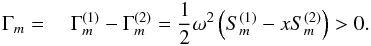 (14)The functions Γm’s are shown in Fig. 1 (see also Fig. 2). Several comments are in order.
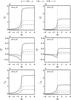 |
Fig. 1 The dimensionless structure functions Γm defined in Eqs. (12b) and (14) vs. Ri. Ri < 0 corresponds to the CZ, while Ri > 0 corresponds to the RZ. For comments, see the text. |
7.1. unstable-stable stratification
In the CZ, x = τ2N2 < 0, Ri < 0 and since  , the last term in (13) has a positive sign. The first term also has a positive sign, and thus the two terms on the rhs in (13) both have a positive sign, which means that they are both of the counter-gradient type. The value of ε is large since the convective flux
  carries almost all the solar flux. Owing to the p dependence exhibited in relation (10d), the value p = 2 corresponds to the case of pure shear (no vorticity).
In the RZ, x = τ2N2 > 0, Ri > 0, we have  . The first term in (13) is of the counter-gradient type, while the second term is up-gradient. At the bottom of the CZ, ε can be related to the power generated by internal gravity waves (Kumar et al. 1999), as already discussed in Eq. (10a) of Paper II. The term
  increases as the rotation curve becomes increasingly flatter (from p = 2 to p = 1), and so does Γm in the first term but its increase is largely cancelled by the decrease in the term ∂Ω / ∂r, which in principle becomes negligible as one approaches the RZ where a rigid body rotation sets in.
7.2. comparison with previous models
It is instructive to compare the momentum diffusivity Km obtained in this work with the one used in the literature. It is usually denoted by Dv (Charbonnel & Talon 2005; Talon & Charbonnel 2005, Eq. (5); Zahn 2008, Eq. (3.5)) 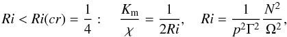 (15)where χ(cm2 s-1) is thermometric conductivity that enters the radiative diffusivity Kr = cpρχ (see Eq. (4d) of Paper I). Several comments about (15) are in order.
The first is about the absence of a factor representing the amount of energy (or power) that creates the mixing. In fact, turbulence is a process that does not generate or destroy energy, rather, it distributes whatever energy is put into the system among a wide variety of scales. Without such an energy, there would be no turbulent motion or, in the presence of turbulence, turning such source of energy off would lead to a decaying turbulent mixing. The well known Kolmogorov law E(k) = Koε2 / 3k − 5 / 3 gives the spectrum of the eddies generated by the nonlinear interaction, but it contains the rate of dissipation or energy input ε which is considered an outside, given variable.
The second comment is about the lack of universality of ε since different stellar interiors have different ε, which then yield different rates of mixing. Thus, the presence of such a factor would ensure that different stars give rise to different states of mixing, as ought to be the case. In the present formalism, one sees from (13) that ε is present and that the dimensionless factor,  (16a)is a measure how much stronger the turbulent diffusivity is than the radiative one represented by χ. The factor (16a) is clearly different for different stars. Third, in (15), the momentum diffusivity is assumed to be a decreasing function of Ri. On the other hand, in the present formalism, the momentum diffusivity can be written in a variety of forms beginning with Eq. (10b) and using (11):
 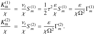 (16b)
Inspection of Figs. 1 shows the basic differences between (15) and (16): a) the function Γm does not decrease with Ri, whereas (15) does and b) (15) is limited to values of Ri < 1 / 4, whereas (16b) embraces any value of Ri. As already discussed in Sect. 7 of Paper I and in Sect. 5 of Paper II, relation (15) assumes the existence of a critical Ri above which there is no mixing, while the most recent data show that such a limit does not exist.
(16b)
Inspection of Figs. 1 shows the basic differences between (15) and (16): a) the function Γm does not decrease with Ri, whereas (15) does and b) (15) is limited to values of Ri < 1 / 4, whereas (16b) embraces any value of Ri. As already discussed in Sect. 7 of Paper I and in Sect. 5 of Paper II, relation (15) assumes the existence of a critical Ri above which there is no mixing, while the most recent data show that such a limit does not exist.
7.3. internal gravity waves
As discussed by the authors cited previously (Kumar & Quataert 1997; Zahn et al. 1997; Kumar et al. 1999; Charbonnel & Talon 2005, 2007), the most recently employed form of the angular momentum equation (Talon & Charbonnel 2005, Eq. (9)), has an additional term due to IGW in the righthand side of Eq. (1f)  (17a)where the explicit form of the IGW luminosity LIGW can be found in the reference above. Its magnitude is approximately 1029 erg s-1 corresponding to 0.004% of the luminosity at the base of the CZ of 2.5 × 1033 erg s-1 (Talon & Charbonnel 2005, Sect. 3.3). From the new equation for the angular momentum, one obtains a time scale of
  (17b)where we used r = 3.5 × 109 cm,ρ = 125 gr cm-3,Ω = 2 × 10⁻⁶ s-1,LIGW = 1029 erg s-1. The value (17b) agrees with the results obtained from more detailed computations discussed in the cited literature. By comparison, if we use the standard Eq. (1a) corresponding to a down-gradient model (DG), we obtain
  (17c)Since the values of Km given in Fig. 14 of Talon & Charbonnel (2005), where Km is called Dv at say the bottom of the CZ, are of the order of 50 cm2 s-1, the τ resulting from (17c) is two-to-three orders of magnitude larger than (17b). Finally, let us take the last term in (13) corresponding to an up-gradient model (UG). We obtain
  (17d)where we have taken ε ≈ 3 × 10⁻⁵ cm2 s-3 that corresponds to LIGW = 1029 erg s-1. Relation (17d) is compatible with the IGW result (17b) if
  (17e)
Figures 1c − d show that this is possible.
(17e)
Figures 1c − d show that this is possible.
8. Conclusions
Given the well known challenge of trying to reproduce the helio data on the solar rotation curve, we have examined the ingredients of the angular momentum equation. It contains two main terms, the Reynolds stresses and the meridional currents which, in a large Re regime such as that characterizing a stellar interior and in a steady state, must balance each other. It is worth noticing that this balance has not yet been exhibited by the numerical simulations published thus far (see Figs. 11 of Brun & Toomre 2002), most probably because they are still too viscous. Since the equations for the meridional currents also depend on the Reynolds stresses, the latter constitute a key ingredient and we have therefore concentrated on how they have been modeled thus far and what the missing terms are that must be included. The final new formula for the Reynolds stress is quite simple, Eq. (4a) and the hope is that it will be tested and assessed to ascertain which angular momentum profiles it produces and what improvement it brings with respect to the expression used thus far, Eq. (1d).
A key feature of the new RSM is that all the relevant equations governing the Reynolds stresses (4a) and the heat and concentration fluxes (5a,b) are obtained by solving linear algebraic equations. This is a welcome feature if one considers the large amount of information that the new model contains: stable stratification, unstable stratification, double-diffusion, differential rotation, shear, radiative losses (arbitrary Peclet number) and meridional currents.
As an illustrative example we have worked out the case of no double diffusion and no meridional currents so as to highlight a key feature of the model. The standard RSM model, based on shear alone, is of the down-gradient type, and it fails to reproduce the helio data that point to a rigid body rotation below the solar convective zone. It was then suggested that IGW, which operate on an up-gradient flux, may be responsible for such a rotational state, and quantitative computations by several authors have confirmed that on a time scale of the order of 107 yrs, the rigid body rotation can be achieved.
Here, we have introduced an alternative that we hasten to stress is not ad hoc but is part and parcel of the RSM model. It is unavoidable and it turns out that the combination vorticity+stable stratification gives rise to an up-gradient term in the Reynolds stresses, which, in the angular momentum equation, produces a characteristic time scale comparable to the one by the IGW model. As Talon & Charbonnel (2005) point out, a mixing model must do more than just reproduce the solar rotation curve and the model presented here must thus await those tests to be performed before a final judgment can be made.
References
- Brummell, N. H., Clune, T. L., & Toomre, J. 2002, ApJ, 570, 825 [Google Scholar]
- Brun, A. S., & Toomre, J. 2002, ApJ, 570, 865 [NASA ADS] [CrossRef] [EDP Sciences] [Google Scholar]
- Canuto, V. M. 2009, Turbulence in astrophysical and geophysical flows, in Interdisciplinary Aspects of Turbulence, Springer Lectures Notes in Physics, ed. W. Hillebrandt, & F. Kupka (Berlin: Springer and Verlag), 2008, 756, 107 [Google Scholar]
- Canuto, V. M., & Dubovikov, M. S. 1998, ApJ, 493, 834 [Google Scholar]
- Canuto, V. M., & Minotti, F. 2001, MNRAS, 328, 829 [NASA ADS] [CrossRef] [Google Scholar]
- Canuto, V. M., Minotti, F., & Shilling, O. 1994, ApJ, 425, 303 [NASA ADS] [CrossRef] [Google Scholar]
- Charbonnel, C., & Talon, S. 2005, Science, 309, 2189 [NASA ADS] [CrossRef] [PubMed] [Google Scholar]
- Charbonnel, C., & Talon, S. 2007, Science, 318, 922 [CrossRef] [PubMed] [Google Scholar]
- Gatski, T. B., & Speziale, C. G. 1993, J. Fluid Mech., 254, 59 [NASA ADS] [CrossRef] [MathSciNet] [Google Scholar]
- Kumar, P., & Quataert, E. J. 1997, ApJ, 475, L143 [NASA ADS] [CrossRef] [Google Scholar]
- Kumar, P., Talon, S., & Zahn, J. P. 1999, ApJ, 520, 859 [NASA ADS] [CrossRef] [Google Scholar]
- Kupka, F. 2009, Turbulence in astrophysical and geophysical flows, in Interdisciplinary Aspects of Turbulence, Springer Lectures Notes in Physics, ed. W. Hillebrandt, & F. Kupka (Berlin: Springer and Verlag), 2008 [Google Scholar]
- Kupka, F., & Muthsam, H. J. 2007, in Convection in Astrophysics, ed. F. Kupka, I. W. Roxburgh, & K. L. Chan (Cambridge Univ. Press), IAU Symp., 239, 86 [Google Scholar]
- Maeder, A., & Maynet, G. 2001, A&A, 373, 555 [NASA ADS] [CrossRef] [EDP Sciences] [Google Scholar]
- Markatos, N. C. 1987, in Encyclopedia of Fluid Mechanics, Complex Phenomena ad Modeling, ed. N. O. Cheremisinoff, London, Gulf, 6, 1221 [Google Scholar]
- Mathis, S., Palacios, A., & Zahn, J. P. 2004, A&A, 425, 243 [NASA ADS] [CrossRef] [EDP Sciences] [Google Scholar]
- Palacios, A., Talon, S., Charbonnel, C., & Forestini, M. 2003, A&A, 399, 603 [NASA ADS] [CrossRef] [EDP Sciences] [Google Scholar]
- Palacios, A., Charbonnel, C., Talon, S., & Seiss, L. 2006, A&A, 453, 261 [NASA ADS] [CrossRef] [EDP Sciences] [Google Scholar]
- Pulkkinen, P., Tuominen, I., Branderburgh, A., et al. 1993, A&A, 267, 265 [NASA ADS] [Google Scholar]
- Talon, S., & Zahn, J. P. 1998, A&A, 329, 315 [NASA ADS] [Google Scholar]
- Talon, S., & Charbonnel, C. 2003, A&A, 405, 1025 [NASA ADS] [CrossRef] [EDP Sciences] [Google Scholar]
- Talon, S., & Charbonnel, C. 2005, A&A, 440, 981 [NASA ADS] [CrossRef] [EDP Sciences] [Google Scholar]
- Taulbee, D. B. 1992, Phys. Fluids, A4, 2555 [NASA ADS] [Google Scholar]
- Thompson, M. J., Christensen-Dalsgaard, J., Miesh, M. S., & Toomre, J. 2003, ARA&A, 41, 599 [NASA ADS] [CrossRef] [Google Scholar]
- Ulrich, R. K., Boyden, J. E., Webster, L., et al. 1988, Sol. Phys., 117, 291 [NASA ADS] [CrossRef] [Google Scholar]
- Virtanen, H. 1989, Ph.D. Thesis, University of Helsinki [Google Scholar]
- Zahn, J. P. 2008, in ed. L. Deng, & K. L.Chan (Cambridge Univ. Press), IAU Symp., 252, 83, 47 [Google Scholar]
- Zahn, J. P., Talon, S., & Matias, J. 1997, A&A, 322, 320 [NASA ADS] [Google Scholar]
All Figures
|
Fig. 1 The dimensionless structure functions Γm defined in Eqs. (12b) and (14) vs. Ri. Ri < 0 corresponds to the CZ, while Ri > 0 corresponds to the RZ. For comments, see the text. |
| In the text | |
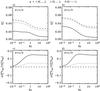 |
Fig. 2 The dimensionless functions Sm in Eq. (10b). |
| In the text | |
Current usage metrics show cumulative count of Article Views (full-text article views including HTML views, PDF and ePub downloads, according to the available data) and Abstracts Views on Vision4Press platform.
Data correspond to usage on the plateform after 2015. The current usage metrics is available 48-96 hours after online publication and is updated daily on week days.
Initial download of the metrics may take a while.