| Issue |
A&A
Volume 519, September 2010
|
|
|---|---|---|
| Article Number | A39 | |
| Number of page(s) | 24 | |
| Section | Interstellar and circumstellar matter | |
| DOI | https://doi.org/10.1051/0004-6361/200913906 | |
| Published online | 09 September 2010 | |
Photoluminescence of hydrogenated amorphous carbons
Wavelength-dependent yield and implications for the extended red emission![[*]](/icons/foot_motif.png)
M. Godard![]() - E. Dartois
- E. Dartois
Institut d'Astrophysique Spatiale (IAS), UMR8617, Université Paris-Sud, bâtiment 121, 91405 Orsay Cedex, France
Received 18 December 2009 / Accepted 11 March 2010
Abstract
Context. Hydrogenated amorphous carbons (a-C:H or HAC) have
proved to be excellent analogs of interstellar dust observed in
galaxies diffuse interstellar medium (DISM) through infrared
vibrational absorption bands (3.4 ![]() m, 6.8
m, 6.8 ![]() m, and 7.2
m, and 7.2 ![]() m
bands). They exhibit photoluminescence (PL) after excitation by
UV-visible photons, and are possible carriers for the extended red
emission (ERE), a broad red emission band observed in various
interstellar environments.
m
bands). They exhibit photoluminescence (PL) after excitation by
UV-visible photons, and are possible carriers for the extended red
emission (ERE), a broad red emission band observed in various
interstellar environments.
Aims. As many candidate materials/molecules can photoluminesce
in the visible, along with the carrier abundance, the
PL efficiency represents one of the strongest constraints set by
such ERE observations. We wish to precisely characterize the
PL behavior of a-C:H as a family of materials.
Methods. The a-C:H samples are produced in the form of films
deposited on substrates by plasma-enhanced chemical vapor deposition.
The produced films were analyzed in transmission by UV-visible and IR
spectroscopy, and the wavelength dependent PL spectra were
recorded. The intrinsic absolute quantum yield ![]() was then rigorously calculated taking self-absorption of the PL by the film and interfaces effects into account.
was then rigorously calculated taking self-absorption of the PL by the film and interfaces effects into account.
Results. A wide range of different laboratory synthesized a-C:H
were analyzed. Their PL properties are dependent on the optical
gap ![]() :
when
:
when ![]() decreases from 4.3 eV to 2.8 eV, the a-C:H vary from highly (
decreases from 4.3 eV to 2.8 eV, the a-C:H vary from highly (
![]() )
yellow photoluminescent soft materials to hard materials that emit a
wider PL band in the red spectral range, with a lower efficiency (
)
yellow photoluminescent soft materials to hard materials that emit a
wider PL band in the red spectral range, with a lower efficiency (
![]() %).
For any given a-C:H, the PL characteristics (central wavelength,
band width and efficiency) are found to be essentially constant over
the explored excitation range (
%).
For any given a-C:H, the PL characteristics (central wavelength,
band width and efficiency) are found to be essentially constant over
the explored excitation range (
![]() nm).
We compared the characteristics of the produced interstellar dust
analog to the constraints imposed by the ERE observations.
nm).
We compared the characteristics of the produced interstellar dust
analog to the constraints imposed by the ERE observations.
Conclusions. As for ERE observations, PL efficiencies
and band widths of a-C:H are both correlated to the PL central
wavelengths. The excitation responsible for the a-C:H emission is
efficient over a wide spectral range that matches the
ERE excitation. The present a-C:H encounter difficulties for the
diffuse ISM ERE observations (
![]() )
in simultaneously satisfying the high quantum yield criteria and
PL spectral characteristics. We still need to investigate the role
of a small number of residual oxygen atoms in the laboratory-produced
a-C:H network in quenching the PL yield, as well as to consider
the interstellar temperature effect for our analogs.
)
in simultaneously satisfying the high quantum yield criteria and
PL spectral characteristics. We still need to investigate the role
of a small number of residual oxygen atoms in the laboratory-produced
a-C:H network in quenching the PL yield, as well as to consider
the interstellar temperature effect for our analogs.
Key words: dust, extinction - radiation mechanisms: non-thermal - infrared: ISM - ISM: lines and bands - astrochemistry - methods: laboratory
1 Introduction
The extended red emission (ERE), first observed in the Red Rectangle nebula (Cohen et al. 1975; Schmidt et al. 1980), is a large (quartile flux width ![]()
![]() between 60 and 120 nm) featureless emission band in the red part
of the visible spectrum (between 540 and 950 nm) observed in a
wide range of astrophysical environments: reflection nebulae (Witt & Boroson 1990; Witt & Schild 1985), carbon-rich planetary nebulae (Furton & Witt 1992,1990), a dark nebula (Mattila 1979; Chlewicki & Laureijs 1987), H II regions (Darbon et al. 2000; Sivan & Perrin 1993; Perrin & Sivan 1992; Darbon et al. 1998), diffuse interstellar medium (DISM) (Szomoru & Guhathakurta 1998; Gordon et al. 1998; Witt et al. 2008), and in external galaxies (Darbon et al. 1998; Pierini et al. 2002; Perrin et al. 1995). ERE is thus a general phenomenon.
between 60 and 120 nm) featureless emission band in the red part
of the visible spectrum (between 540 and 950 nm) observed in a
wide range of astrophysical environments: reflection nebulae (Witt & Boroson 1990; Witt & Schild 1985), carbon-rich planetary nebulae (Furton & Witt 1992,1990), a dark nebula (Mattila 1979; Chlewicki & Laureijs 1987), H II regions (Darbon et al. 2000; Sivan & Perrin 1993; Perrin & Sivan 1992; Darbon et al. 1998), diffuse interstellar medium (DISM) (Szomoru & Guhathakurta 1998; Gordon et al. 1998; Witt et al. 2008), and in external galaxies (Darbon et al. 1998; Pierini et al. 2002; Perrin et al. 1995). ERE is thus a general phenomenon.
This spectral feature is commonly attributed to the photoluminescence (PL) of interstellar dust following the absorption of UV-visible photons, but the true nature of the ERE carriers is still under debate. Many candidates have been proposed over the past decades: polycyclic aromatic hydrocarbon (PAH) molecules, ions or clusters (Berné et al. 2008; D'Hendecourt et al. 1986; Vijh et al. 2005; Rhee et al. 2007), hydrogenated amorphous carbons (HAC or a-C:H) (Seahra & Duley 1999; Witt & Boroson 1990; Furton & Witt 1993; Witt & Schild 1988; Duley et al. 1997; Duley 1985; Duley & Williams 1988), quenched carbonaceous composites (QCC) (Wada et al. 2009; Sakata et al. 1992), nanodiamonds (Duley 1988; Chang et al. 2006), C60 (Webster 1993), and also non carbon-based materials such as crystalline silicon nanoparticules (SNP) (Ledoux et al. 2001; Witt et al. 1998; Ledoux et al. 1998; Smith & Witt 2002). Recently, Duley (2009) have suggested that ERE may not be exclusively caused by PL but may result from a combination of PL and carbon clusters/dehydrogenated carbon molecules thermal emission. Up to now, none of these candidates have been clearly identified as the ERE carrier material.
To identify which interstellar material is responsible for this
observed large emission band, or, at least, narrow the range of
candidates, each constraint imposed by the ERE observations must
be carefully compared to the properties of ERE carrier candidates.
An example of an observational relationship that should help identify
the ERE carriers is the correlation found between the width and
peak wavelength of ERE (Darbon et al. 1999; Witt & Boroson 1990): the band width ![]() increases from 60 to 120 nm as the ERE maximum position
varies from 650 to 780 nm. In addition to the ERE positions
and shapes, the observational constraints, reviewed by Smith & Witt (2002) and Witt & Vijh (2004), set a lower limit on the PL quantum yield of the ERE. This quantum yield
increases from 60 to 120 nm as the ERE maximum position
varies from 650 to 780 nm. In addition to the ERE positions
and shapes, the observational constraints, reviewed by Smith & Witt (2002) and Witt & Vijh (2004), set a lower limit on the PL quantum yield of the ERE. This quantum yield ![]() is defined as the ratio of the emitted and the absorbed (by the
ERE carriers) photon numbers. This yield is the quantum yield and
must not be confused with the yield defined as an energy ratio. The
quantum yield can be greater than one in the case of more than one
ERE photon emission after an UV-visible photon absorption. It is
not straightforward to evaluate the ERE quantum yield from
observations (Smith & Witt 2002).
Some hypothesis have to be assumed about the excitation range that
causes the ERE and the way the amount of absorbed light is
determined from dust-scattered light (i.e. assuming the dust albedo and
extinction law wavelength dependence, the illuminating star's spectral
energy distribution and the geometry of the nebula as well known
parameters). The determined absorption accounts for all kinds of
intervening molecules and solids, not only ERE carriers. Thus, the
observed quantum yields set a lower limit on the ERE efficiency.
The efficiency lower limits reviewed by Smith & Witt (2002)
lie between about 0.1% and up to 10% depending on the interstellar
environments (quantum efficiency as high as 20% have been estimated by
the same method for ERE in the Red Rectangle nebula,
which is treated apart). They find that ERE efficiency tends to
decline with the increase of local radiation field intensity.
is defined as the ratio of the emitted and the absorbed (by the
ERE carriers) photon numbers. This yield is the quantum yield and
must not be confused with the yield defined as an energy ratio. The
quantum yield can be greater than one in the case of more than one
ERE photon emission after an UV-visible photon absorption. It is
not straightforward to evaluate the ERE quantum yield from
observations (Smith & Witt 2002).
Some hypothesis have to be assumed about the excitation range that
causes the ERE and the way the amount of absorbed light is
determined from dust-scattered light (i.e. assuming the dust albedo and
extinction law wavelength dependence, the illuminating star's spectral
energy distribution and the geometry of the nebula as well known
parameters). The determined absorption accounts for all kinds of
intervening molecules and solids, not only ERE carriers. Thus, the
observed quantum yields set a lower limit on the ERE efficiency.
The efficiency lower limits reviewed by Smith & Witt (2002)
lie between about 0.1% and up to 10% depending on the interstellar
environments (quantum efficiency as high as 20% have been estimated by
the same method for ERE in the Red Rectangle nebula,
which is treated apart). They find that ERE efficiency tends to
decline with the increase of local radiation field intensity.
Amorphous hydrogenated carbons (a-C:H or HAC) are one of the
ERE carrier candidates. They are carbonaceous material consisting
of a mixture of sp2 and sp3
hybridized bonds. The a-C:H are of astrophysical interest since they
have proved to be analogs of one of the interstellar dust components
(e.g. Dartois et al. 2005; Sandford et al. 1991; Spoon et al. 2004; Pendleton & Allamandola 2002) through IR absorption bands (C-H stretching modes at 3.4 ![]() m and C-H bending modes at 6.85 and 7.25
m and C-H bending modes at 6.85 and 7.25 ![]() m)
ubiquitously observed in the diffuse interstellar medium of both our
Galaxy and of other galaxies. This material represents a highly
significant dust component of galaxies, since 5 to 30% of the total
available cosmic carbon (Dartois et al. 2005; Sandford et al. 1991; Duley et al. 1998) is contained in the 3.4
m)
ubiquitously observed in the diffuse interstellar medium of both our
Galaxy and of other galaxies. This material represents a highly
significant dust component of galaxies, since 5 to 30% of the total
available cosmic carbon (Dartois et al. 2005; Sandford et al. 1991; Duley et al. 1998) is contained in the 3.4 ![]() m feature carrier.
m feature carrier.
Amorphous hydrogenated carbons photoluminesce in the visible spectral range. Characterization of the photoluminescence behavior of this interstellar component is thus required to evaluate its contribution to the interstellar dust emission, and it is especially important to compare the a-C:H PL to the ERE observed properties. In particular, the PL efficiency, which is one of the strongest constraints set by the observations for the ERE carrier candidates as described above, has to be accurately investigated for the a-C:H materials. Until now, most of the works about the photoluminescence efficiencies of astrophysical relevant a-C:H provided results in terms of relative efficiencies (e.g. Rusli et al. 1996) and only for a few excitation wavelengths. The few results for absolute a-C:H PL efficiencies (Ledoux et al. 2001; Furton & Witt 1993; Furton et al. 1999) vary over four orders of magnitude. In addition, optical effects modifying the apparent efficiency as compared to the intrinsic efficiency are not properly taken into account.
Carefully studying the PL absolute efficiency of amorphous hydrogenated carbons is the aim of this work. In this article, we present the first results of a systematic a-C:H photoluminescence study, which has the advantage of being a multi-wavelength excitation study that properly takes optical effects in the emitting thin film into account. We describe in Sect. 2 the experimental setups allowing the production and analysis of the a-C:H samples. Section 3 describes how the a-C:H PL absolute quantum yield is calculated from the PL measurements (detailed calculations in appendixes) and the obtained results (concerning PL yields and spectra) are put in perspective with previous relative efficiencies measurements in Sect. 4. These results and their astrophysical implications about ERE are then discussed in Sect. 5, followed by our conclusion in Sect. 6.
2 Experiments
2.1 Film preparation
The interstellar a-C:H analogs were produced using a plasma-enhanced chemical vapor deposition (PECVD) system: a plasma of a hydrocarbon precursor gas is created in a vacuum chamber. The pressure during deposition was maintained in the range between 10-3 and 10-1 mbar. As the precursor gas, we used different hydrocarbons (methane, acetylene, butadiene, phenylacetylene, isobutane, toluene, and limonene) that can also be mixed with molecular hydrogen or argon. The addition of an inert gas diluent such as argon allows us to stabilize the plasma or to change deposition conditions (Seth & Babu 1993). The C/H ratio and the hybridization type vary from one hydrocarbon precursor to another one and have some influence on the produced a-C:H (Schwarz-Selinger et al. 1999).
The plasma is created via an Evenson cavity used to excite microwave discharges in molecular precursors with a 2450 MHz radio-frequency microwave generator. The film is formed by deposition of the radicals and ions resulting from the precursor on a substrate (quartz or KBr, for example) located in the vacuum chamber. A negative electric potential can be applied to a grid placed just in front of the substrate in order to accelerate the ions coming from the plasma. By applying different voltages, thus varying the energy of the impinging ions, we can explore a wider range of produced a-C:H films (Rusli et al. 1996; Schwarz-Selinger et al. 1999). The deposition time to obtain a few micrometers thick film is variable, from a few minutes to a few hours depending on the deposition conditions. The a-C:H film obtained can then be analyzed ex-situ.
2.2 Film characterization: structure and optical constants
![\begin{figure}
\par\includegraphics[width=8.8cm,clip]{13906fg1a}\hspace*{4mm}
\includegraphics[width=8.8cm,clip]{13906fg1b}
\vspace*{2mm}
\end{figure}](/articles/aa/full_html/2010/11/aa13906-09/img21.png)
|
Figure 1: Examples of transmission spectra in the UV-visible (left) and IR region (right) of a typically produced a-C:H film. |
| Open with DEXTER | |
2.2.1 Infrared spectroscopy
The IR ex situ analysis of the samples were performed either by FTIR spectroscopy with a Bruker IFS66V infrared spectrometer or by FTIR micro-spectroscopy using a Nicolet Magna-IR 560 ESP spectrometer coupled to a Nicolet Nicplan infrared microscope located at the synchrotron SOLEIL (the microscope enables us to check the sample planarity). The transmission spectra were recorded in the 7500-400 cm-1 range (when using KBr as substrate) with a resolution of 2 cm-1. An example of produced a-C:H IR spectrum of the a-C:H produced is presented on the right panel of Fig. 1.Table 1: a-C:H vibrational assignments.
The infrared transmission spectrum and its absorption bands give us access to the structure of the a-C:H produced. Table 1 presents the assignment of the prominent bands observed in the film spectra (e.g. Dartois et al. 2005; Ristein et al. 1998; Dartois et al. 2004).
Interference fringes appear in the infrared transmission spectra,
resulting from the multiple reflections at the film interfaces. These
fringes can give us information about the thickness and the optical
constants of the film necessary to the PL study. In the region
devoid of absorption, the interfringe
![]() (in cm-1) is a function of the sample thickness H and of its refraction index n0:
(in cm-1) is a function of the sample thickness H and of its refraction index n0:

Alternatively, for thin films, the
2.2.2 UV-visible spectroscopy
The UV-visible transmission spectra of a-C:H film deposited onto a quartz substrate (see left of Fig. 1) are measured in the spectral range between 210 nm and 710 nm with a 2 nm resolution, using an Avalight DS-DUV deuterium lamp and a fibered Avaspec-2048 Czerny-Turner grating spectrometer.
With this transmission spectrum and the film thickness obtained
with the IR spectrum, we can establish a first-order UV-visible
imaginary part
![]() of the a-C:H complex index or the film absorption coefficient
of the a-C:H complex index or the film absorption coefficient
![]() in this range. These parameters are linked to the transmittance
in this range. These parameters are linked to the transmittance
![]() measurements by Eq. (2) and are needed to evaluate the PL yield:
measurements by Eq. (2) and are needed to evaluate the PL yield:
![]() will allow us to evaluate how the incident excitation (giving rise to
the photoluminescence) is absorbed by the sample and how it is
distributed in the film:
will allow us to evaluate how the incident excitation (giving rise to
the photoluminescence) is absorbed by the sample and how it is
distributed in the film:
![\begin{displaymath}
T(\lambda) = {\rm exp} \left[-\alpha(\lambda)\ H \right] = {...
...xp} \left[- \frac{4 \pi}{\lambda}\ \kappa(\lambda)\ H \right].
\end{displaymath}](/articles/aa/full_html/2010/11/aa13906-09/img30.png)
We can then determine the a-C:H optical gap, often defined in the literature by
2.2.3 Refractive index determination
The real part of the sample refractive index n0 is estimated from the sample optical gap ![]() because these both parameters are correlated. We brought together in Fig. 2
a-C:H refractive indexes and optical gaps data from different studies
(see references in caption). When the optical gap is given by
because these both parameters are correlated. We brought together in Fig. 2
a-C:H refractive indexes and optical gaps data from different studies
(see references in caption). When the optical gap is given by
![]() (red point in Fig. 2), we add 0.6 eV to infer the
(red point in Fig. 2), we add 0.6 eV to infer the ![]() gap. This well seen correlation between n0 and
gap. This well seen correlation between n0 and ![]() gives refractive indexes between 1.25 and 1.85 for our a-C:H samples.
gives refractive indexes between 1.25 and 1.85 for our a-C:H samples.
![\begin{figure}
\par\includegraphics[width=8.8cm,clip]{13906fg2}
\end{figure}](/articles/aa/full_html/2010/11/aa13906-09/img35.png)
|
Figure 2:
Refractive index of different a-C:H samples as a function of the optical gap (obtained by Bubenzer et al. 1983; Bourée et al. 1998; Choi 2001; Silva et al. 1996; Furton et al. 1999; Lazar 1998; Wagner & Lautenschlager 1986; Dischler et al. 1983; and Kassavetis et al. 2007). For data in red, only the
|
| Open with DEXTER | |
Information about n0 can also be found in the interferences pattern of the IR transmission spectra (Swanepoel 1983). We compared the refractive index estimated for few a-C:H samples from the IR spectra obtained by micro-spectroscopy to the one found from the optical gap, and a good agreement exists between these methods.
2.2.4 sp2/sp3 ratio determination
Carbon atoms in a-C:H exist in both sp2 and sp3 electronic configurations. The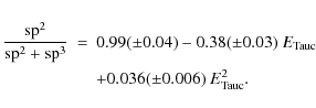
To obtain information about the structure of our a-C:H materials, we estimated the sp2 fraction from this relation and the optical gaps we measured. For our samples, sp2/sp3 ratios are found between 5% and 30%.
![\begin{figure}
\par\includegraphics[width=8.8cm,clip]{13906fg3}
\end{figure}](/articles/aa/full_html/2010/11/aa13906-09/img39.png)
|
Figure 3: sp2 fraction of different a-C:H samples as a function of the Tauc optical gap (obtained by Robertson 1996; Kleber 1991; Jarman et al. 1986; Tamor & Vassell 1994; and Kassavetis et al. 2007). The colored area corresponds to the Dartois et al. (2005) a-C:H sample (see text for details). Extreme cases of glassy carbon (Robertson 1986; Turlo & Rozwadowskajasniewska 1987), graphite (all sp2) (filled squares), and diamond (all sp3) (filled diamond) are also represented. The dashed line is a second-degree polynomial fit to these data. |
| Open with DEXTER | |
2.3 Photoluminescence measurements
To quantitatively measure the photoluminescence of our produced films,
we have at our disposal a double monochromator (for excitation and
emission) Perkin Elmer LS55 luminescence spectrometer coupled to a
front surface device. It allows us to measure the photoluminescence of
the a-C:H between 200 nm and 800 nm. The photoluminescence of
the sample is measured ex-situ at room temperature just after its
production. The external medium during this measurement, designed by
the subscript 1, is the air. The quasi-monochromatic excitation
(excitation
![]() nm)
of the samples occurs at UV-visible wavelengths greater than
200 nm but quantitative measurements are possible for excitation
wavelength greater than 250 nm (
nm)
of the samples occurs at UV-visible wavelengths greater than
200 nm but quantitative measurements are possible for excitation
wavelength greater than 250 nm (![]() 5 eV), using the xenon flash lamp of the LS55. The excitation angle
5 eV), using the xenon flash lamp of the LS55. The excitation angle
![]() and the emission detection angle
and the emission detection angle
![]() (from the sample surface normal) are performed at 30 and -60 degrees,
respectively, to get rid of any specular reflexion. We use almost
perfect Lambertian reflectance standards (Labsphere Spectralon diffuse
reflectance standards) as reference to measure the incident excitation
flux at the location of the sample as well as the relative instrument
response.
(from the sample surface normal) are performed at 30 and -60 degrees,
respectively, to get rid of any specular reflexion. We use almost
perfect Lambertian reflectance standards (Labsphere Spectralon diffuse
reflectance standards) as reference to measure the incident excitation
flux at the location of the sample as well as the relative instrument
response.
For absolute calibration purposes, we replace the front assay
device by a Labsphere integrating sphere coupled to the LS55
luminescence spectrometer with optic fibers in order to provide a
second and independent measurement of absolute PL yield. This set
up was used to build our own PL standard to check the validity of
our absolute quantum yield calculation (explained in the next section).
A bismuth germanate crystal (
![]() ,
BGO hereafter) window of the same shape as our substrate was used as
PL standard. BGO PL yield is high, remains stable, and can be
easily manipulated. Moreover, because of its high Stokes' shift, there
is no overlap of the absorption and emission spectra (re-absorption of
the emission by the sample being not easily considered when using an
integrating sphere).
,
BGO hereafter) window of the same shape as our substrate was used as
PL standard. BGO PL yield is high, remains stable, and can be
easily manipulated. Moreover, because of its high Stokes' shift, there
is no overlap of the absorption and emission spectra (re-absorption of
the emission by the sample being not easily considered when using an
integrating sphere).
3 Determination of the absolute intrinsic photoluminescence quantum yield
3.1 With the luminescence spectrometer
The intrinsic quantum yield determination requires perfect knowledge
of the optical effects implied in the measurement. The detailed
calculations are presented in Appendices A and B,
and we summarize here the steps needed to retrieve this yield. In the
appendixes, the emission of light from a thin film is modeled and the
interference effects of the reflections on the interfaces of the film
are calculated (Holm et al. 1982; Nollau et al. 2000; Lukosz 1981).
The thin film is an absorbing dielectric layer (the subscript 0 is used
to design this medium) located between two different media 1 (the
external medium) and 2 (the substrate). The luminescent centers
are assumed to be electric dipole sources with randomly oriented dipole
moment ![]() .
.
We consider the light transmitted outside the film (i.e. in medium 1) separated into two beams: the direct beam D is the one emitted directly in the direction of medium 1 toward the detector, and the reflected beam R
is the beam that is first directed toward the substrate (i.e. medium 2)
and reflected off the back surface of the film (i.e. interface 0/2)
before being transmitted in medium 1. The emission angles in the film
of the D and R beams are thus
![]() and
and
![]() ,
respectively, from the sample surface normal (figures of this geometry exist in the appendixes). The angle
,
respectively, from the sample surface normal (figures of this geometry exist in the appendixes). The angle
![]() is given by the observation angle in medium 1,
is given by the observation angle in medium 1,
![]() ,
and the Snell-Descartes refraction law. Each of these beams is
reflected many times between each interface of the film and will
influence the measured yield with respect to the intrinsic one.
,
and the Snell-Descartes refraction law. Each of these beams is
reflected many times between each interface of the film and will
influence the measured yield with respect to the intrinsic one.
The expressions of these beams amplitude account for the
eventual self-absorption of the emission by the film from the emitting
dipole location to medium 1 (considered non-absorbing), calculated from
the absorption coefficient (the self-absorption being expressed by
![]() in relation 6).
in relation 6).
Both of these beams undergo losses when they are transmitted out of the
film or reflected inside the film. These losses are expressed through
the Fresnel coefficients,
![]() and
and
![]() ,
expressed for complex indexes in Appendix C. For example, the transmittance of the emitted power at the interface between a-C:H material and air is
,
expressed for complex indexes in Appendix C. For example, the transmittance of the emitted power at the interface between a-C:H material and air is
|
(3) |
There is also a significant modification of the radiant intensity between media 0 and 1 because of the modification at the interface of the solid angle under which the emission is detected. This modification is expressed by the ratio of infinitesimal solid angles in each medium (Appendix B):
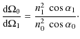
|
(4) |
The reflections at the film interfaces of each beam create an interference effect called the multiple-reflections interference effect. The superposition of the D and R beams (whose directions of emission form an angle equals to
The emitted photoluminescence power is proportional to the power of absorbed light and to the photoluminescence efficiency
![]() .
The power absorbed by the film at the depth h on a thickness
.
The power absorbed by the film at the depth h on a thickness ![]() is
is
![]() and the radiant intensity (in W/sr) emitted by this film thickness is then
and the radiant intensity (in W/sr) emitted by this film thickness is then
![]() .
The resulting emission of this monochromatic absorption is shared out
on a range of visible wavelengths according to a normalized
.
The resulting emission of this monochromatic absorption is shared out
on a range of visible wavelengths according to a normalized![]() emission profile
emission profile
![]() .
The determination of the absorption profile
.
The determination of the absorption profile ![]() (as a function of the film depth h and of the excitation wavelength
(as a function of the film depth h and of the excitation wavelength
![]() )
results from the absorption coefficient
)
results from the absorption coefficient
![]() calculated from the UV-visible transmission spectrum (see Sect. 2.2.2) and the incident excitation power on the sample
calculated from the UV-visible transmission spectrum (see Sect. 2.2.2) and the incident excitation power on the sample
![]() :
:
| |
= | ![$\displaystyle -\ {\rm d}\left(T_{10}(\lambda_{\rm exc})\ \exp \left[ -\ \frac{\...
...mbda_{\rm exc})\ h}{\cos \alpha_{\rm exc, 0}} \right]\ P_{\rm incident} \right)$](/articles/aa/full_html/2010/11/aa13906-09/img63.png)
|
|
| = | ![$\displaystyle T_{10}(\lambda_{\rm exc})\ \frac{\alpha(\lambda_{\rm exc})\ {\rm ...
...pha(\lambda_{\rm exc})\ h}{\cos \alpha_{\rm exc, 0}} \right]\ P_{\rm incident}.$](/articles/aa/full_html/2010/11/aa13906-09/img64.png)
|
(5) |
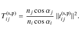
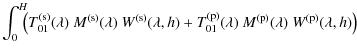
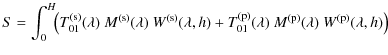
A complete calculation done in the appendixes shows that the specific radiant intensity
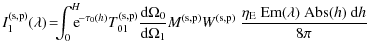
where
where ni and
The emitted specific power detected by the LS55 instrument in the solid angle ![]() (after correction by the instrument response) is
(after correction by the instrument response) is
| (7) |
With
The photoluminescence efficiency
![]() ,
defined as a ratio of energy or power, is then obtained:
,
defined as a ratio of energy or power, is then obtained:
| |
= | (8) |
where
| |
= | 
|
|
In most astrophysical papers about the extended red emission, the yield of this observed emission feature is given as a quantum yield, i.e., a ratio of photons numbers, whereas we measure the energy. To do this conversion, the energy has to be multiplied by
Taking all these optical effects into account allows us to obtain the intrinsic and absolute photoluminescence quantum yield of our a-C:H material, instead of an external yield that can appear significantly lower than the intrinsic efficiency when these effects are neglected.
The variable
![]() is obtained from the power detected by the instrument
is obtained from the power detected by the instrument
![]() corrected by
corrected by
![]() ,
the instrument response between the sample and the detector:
,
the instrument response between the sample and the detector:
![]() .
A Labsphere Spectralon Lambertian reflectance standard used at the
sample location allows us to measure the true incident excitation
.
A Labsphere Spectralon Lambertian reflectance standard used at the
sample location allows us to measure the true incident excitation
![]() .
The reflectance
.
The reflectance
![]() of this standard is known. The radiant intensity diffused by the Lambertian standard in the direction given by
of this standard is known. The radiant intensity diffused by the Lambertian standard in the direction given by ![]() from the surface normal is
from the surface normal is
![]() .
Thus,
.
Thus,
![]() is linked to the measurement
is linked to the measurement
![]() by the relation:
by the relation:
| (10) |
It should be noted that, in this description allowing us to calculate the PL efficiency, we do not take the secondary PL emission, i.e., the PL emission by the sample following the self-absorption of a previous PL photon, into account. We only take the self-absorption into account, not the eventual additional PL that could result of this self-absorption. As pointed out by Malloci et al. (2004), the contribution of this additional emission is very small. Moreover, this secondary photoluminescence can occur only when there is a superposition of the absorption and emission bands. This superposition is weak for our samples. Therefore, the obtained PL yields when neglecting the secondary PL are not significantly overestimated.
3.2 With the integrating sphere: validation of the absolute yield determination
To check the validity of the model described above and used to
determine the PL absolute yields of our a-C:H samples, we
determined the PL absolute quantum yield of a BGO sample by two
independent methods. The first one is the method described in
Sect. 3.1
and also used for a-C:H samples (media 0 and 2 being both BGO as there
is no substrate for this sample), and the other one results from a
measurement with an integrating sphere (using the excitation and the
detection blocks of the luminescence spectrometer). The
PL absolute yield when using an integrating sphere is determined
with the method given in De Mello et al. (1997).
The results found by both methods, presented in Fig. 4, are in good agreement. These absolute values are also similar to the one found in Rodnyi (1997) and Weber & Monchamp (1973) (
![]() at 295 K). This validates our method for calculating absolute internal yield from film photoluminescence measurement with the luminescence spectrometer.
at 295 K). This validates our method for calculating absolute internal yield from film photoluminescence measurement with the luminescence spectrometer.
4 Results
![\begin{figure}
\par\includegraphics[width=9cm,clip]{13906fg4}
\vspace*{6mm}
\end{figure}](/articles/aa/full_html/2010/11/aa13906-09/img102.png)
|
Figure 4: BGO absolute PL quantum yield for different excitation wavelengths, determined by two independent methods: with a front surface device (crosses) or with an integrating sphere (circles). The variation with excitation of PL intensity (i.e. relative efficiencies) found in Weber & Monchamp (1973) is also displayed for comparison (solid line). |
| Open with DEXTER | |
![\begin{figure}
\par\includegraphics[width=9cm,clip]{13906fg5}
\vspace*{5.5mm}
\end{figure}](/articles/aa/full_html/2010/11/aa13906-09/img103.png)
|
Figure 5:
Examples of the photoluminescence spectra of an a-C:H sample, for different excitation wavelengths (
|
| Open with DEXTER | |
The produced a-C:H samples are yellow orange films (at visible light),
with a thickness varying typically from 0.5 to 10 microns. The
photoluminescence of these films seen under an UV lamp (optical
engineering's model 22-UV) has an apparent color varying from yellow to
red. We display in Fig. 5
an example of an a-C:H sample photoluminescence spectrum measured for
different excitation wavelengths ranging from 250 to 490 nm. The
PL color of this sample under the UV lamp appears yellow to the
eye. The photoluminescence is a broad and featureless band. The
PL band does not seem to shift with varying excitation energy
except when the excitation occurs for wavelengths corresponding to
those of the PL band: in such cases, the PL band moves to
greater wavelengths (since
![]() )
and its intensity decreases until the emission does not occur at all
because the excitation goes out of the absorption band (as seen in
Fig. 1).
)
and its intensity decreases until the emission does not occur at all
because the excitation goes out of the absorption band (as seen in
Fig. 1).
![\begin{figure}
\par\includegraphics[width=8.8cm,clip]{13906fg6}
\vspace*{4mm}
\end{figure}](/articles/aa/full_html/2010/11/aa13906-09/img105.png)
|
Figure 6:
Variation in the a-C:H photoluminescence color with the material optical gap
|
| Open with DEXTER | |
The PL color changes with the optical gap of the material, but also the PL efficiency. In Fig. 7, we can see that the absolute quantum yield of our a-C:H samples decreases from about 3% to 0.01% when ![]() varies
from 4.3 to 2.8 eV. Previous studies from other groups (see
references in caption) give a-C:H PL relative efficiency results
and the exponential decrease of the relative efficiency with the
optical gap agrees with our results. We converted these relative
quantum yields into absolute ones by adjusting the whole of them to our
absolute values. Then, a-C:H PL absolute yields are obtained on a
wider range of optical gaps than with only our samples. The exponential
fit of these data gives an absolute quantum yield variation with the
varies
from 4.3 to 2.8 eV. Previous studies from other groups (see
references in caption) give a-C:H PL relative efficiency results
and the exponential decrease of the relative efficiency with the
optical gap agrees with our results. We converted these relative
quantum yields into absolute ones by adjusting the whole of them to our
absolute values. Then, a-C:H PL absolute yields are obtained on a
wider range of optical gaps than with only our samples. The exponential
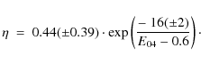
fit of these data gives an absolute quantum yield variation with the ![]() optical gap (in eV) with the following equation (the 3
optical gap (in eV) with the following equation (the 3![]() uncertainty estimation for the fit parameters are indicated and corresponds to the dotted lines in Fig. 7):
uncertainty estimation for the fit parameters are indicated and corresponds to the dotted lines in Fig. 7):
The PL quantum yield can also be linked to the estimated sp2 fraction as shown in Fig. 8. Figures 7 and 8 show exponential fits that correspond to an equation of the form
![\begin{figure}
\par\includegraphics[width=8.8cm,clip]{13906fg7}
\end{figure}](/articles/aa/full_html/2010/11/aa13906-09/img110.png)
|
Figure 7:
Variation in the a-C:H absolute photoluminescence quantum yield |
| Open with DEXTER | |
![\begin{figure}
\par\includegraphics[width=8.8cm,clip]{13906fg8}
\end{figure}](/articles/aa/full_html/2010/11/aa13906-09/img111.png)
|
Figure 8:
Variation in the a-C:H absolute photoluminescence quantum yield |
| Open with DEXTER | |
With Figs. 6 and 7
together, we can deduce that the PL yield decreases when the
photoluminescence central wavelength increases. This is shown in
Fig. 9: a-C:H emission
varies from yellow highly efficient PL to red and lower efficient
PL when the gap decreases. This corresponds to a PL central
wavelength range between 460 and 660 nm. One can see in
Fig. 10 that the width of the band ![]() is correlated to the PL color and increases from about 60 to 210 nm (i.e FWHM
is correlated to the PL color and increases from about 60 to 210 nm (i.e FWHM
![]() nm) when the band moves to longer wavelengths.
nm) when the band moves to longer wavelengths.
![\begin{figure}
\par\includegraphics[width=8.8cm,clip]{13906fg9}
\end{figure}](/articles/aa/full_html/2010/11/aa13906-09/img113.png)
|
Figure 9:
Variation in the a-C:H photoluminescence quantum yield |
| Open with DEXTER | |
![\begin{figure}
\par\includegraphics[width=8.8cm,clip]{13906fg10}
\end{figure}](/articles/aa/full_html/2010/11/aa13906-09/img114.png)
|
Figure 10:
Variation in the a-C:H photoluminescence band width |
| Open with DEXTER | |
The influence of the excitation wavelength on the a-C:H photoluminescence is shown in Figs. 11 and 12. In Fig. 11,
the PL central wavelength is plotted as a function of the
excitation wavelength for different samples. The PL band position
does not vary with
![]() ,
except when the excitation occurs in the PL band (i.e., to the
right of the dotted line) since the emission energy is necessarily
lower than the excitation energy. When this situation happens, light is
emitted only in the high-wavelength part of the PL band, and the
PL central wavelength decays to a redder color as observed in
Figs. 11 and 5.
,
except when the excitation occurs in the PL band (i.e., to the
right of the dotted line) since the emission energy is necessarily
lower than the excitation energy. When this situation happens, light is
emitted only in the high-wavelength part of the PL band, and the
PL central wavelength decays to a redder color as observed in
Figs. 11 and 5.
![\begin{figure}
\par\includegraphics[width=8.8cm,clip]{13906fg11}
\end{figure}](/articles/aa/full_html/2010/11/aa13906-09/img116.png)
|
Figure 11:
Variation in the a-C:H photoluminescence central wavelength with the
excitation wavelength for different a-C:H samples, represented with
different colors and symbols linked by lines as guides for the eye. The
dashed line represents the equation
|
| Open with DEXTER | |
In the explored range, the excitation energy does not seem to have a strong influence on the PL color but also on the PL efficiency as shown in Fig. 12. The absolute quantum yield as a function of the excitation wavelength is almost constant.
![\begin{figure}
\par\includegraphics[width=8.8cm,clip]{13906fg12}
\end{figure}](/articles/aa/full_html/2010/11/aa13906-09/img117.png)
|
Figure 12: Variation in the a-C:H photoluminescence yield with the excitation wavelength for different a-C:H samples, represented with different colors and symbols linked by lines as guides for the eye. |
| Open with DEXTER | |
5 Discussion
5.1 Photoluminescence spectra
To compare the photoluminescence of our a-C:H with extended red emission observations, we display the PL width ![]() (and the FWHM) in Fig. 13 as a function of the emission peak wavelength
(and the FWHM) in Fig. 13 as a function of the emission peak wavelength
![]() ,
of both a-C:H laboratory samples and ERE observations. The a-C:H PL data are those presented in Fig. 10 of this paper, together with data from Lin & Feldman (1982), Lin & Feldman (1983), Watanabe et al. (1982), Wagner & Lautenschlager (1986), Chernyshov et al. (1991), Xu et al. (1993), Rusli et al. (1996), Ledoux et al. (2001), and Dartois et al. (2005). The ERE observations data are taken from Fig. 1 in Darbon et al. (1999),
which regrouped most of the ERE spectral observations. We also add
the ERE observations corresponding to the DISM (Szomoru & Guhathakurta 1998) and L780 dark nebula (Mattila 1979) for which the width and central wavelength determination are much less constrained.
,
of both a-C:H laboratory samples and ERE observations. The a-C:H PL data are those presented in Fig. 10 of this paper, together with data from Lin & Feldman (1982), Lin & Feldman (1983), Watanabe et al. (1982), Wagner & Lautenschlager (1986), Chernyshov et al. (1991), Xu et al. (1993), Rusli et al. (1996), Ledoux et al. (2001), and Dartois et al. (2005). The ERE observations data are taken from Fig. 1 in Darbon et al. (1999),
which regrouped most of the ERE spectral observations. We also add
the ERE observations corresponding to the DISM (Szomoru & Guhathakurta 1998) and L780 dark nebula (Mattila 1979) for which the width and central wavelength determination are much less constrained.
![\begin{figure}
\par\includegraphics[width=8.8cm,clip]{13906fg13}
\vspace*{5mm}
\end{figure}](/articles/aa/full_html/2010/11/aa13906-09/img118.png)
|
Figure 13:
Comparison between spectral characteristics (band width and central
wavelength) of ERE (red filled squares) and a-C:H PL (black
filled circles for our measurements and blue other symbols for a-C:H
PL data coming from previous studies (Watanabe et al. 1982; Rusli et al. 1996; Ledoux et al. 2001; Dartois et al. 2005; Lin & Feldman 1982; Xu et al. 1993; Wagner & Lautenschlager 1986; Lin & Feldman 1983; Chernyshov et al. 1991)). The ERE observations data come from Fig. 1 in Darbon et al. (1999), and we add the ERE observations corresponding to the DISM (Szomoru & Guhathakurta 1998) (square with both |
| Open with DEXTER | |
It should be noted that the ERE spectral characteristics in DISM
seem different from the other ERE detections: ERE in the DISM
appears to occur at shorter wavelengths than in other environments and
with a wider PL band. Szomoru & Guhathakurta (1998) detected an ERE spectrum centered on 600 nm, whereas
![]() are between 650 and 700 nm in reflection nebulae (e.g. Witt & Boroson 1990), around 700 nm in the dusty halo of M 82 (Perrin et al. 1995), between 700 and 780 nm in planetary nebulae (Furton & Witt 1992,1990) and HII regions (Darbon et al. 2000; Sivan & Perrin 1993; Perrin & Sivan 1992; Darbon et al. 1998) and seems to be even above 800 nm in the Evil Eye galaxy (Pierini et al. 2002). Another ERE observation in high galactic latitude interstellar clouds made by Witt et al. (2008) (not plotted in Fig. 13
because no reliable width can be determined) seems to confirm that, in
the DISM, the ERE emission peak wavelength lies around
600 nm. As will be discussed in the next section, the DISM
ERE observations are difficult and few, but if these detections
are confirmed by future DISM observations, it shows the specific
conditions and/or carriers of ERE in the diffuse interstellar
medium environments.
are between 650 and 700 nm in reflection nebulae (e.g. Witt & Boroson 1990), around 700 nm in the dusty halo of M 82 (Perrin et al. 1995), between 700 and 780 nm in planetary nebulae (Furton & Witt 1992,1990) and HII regions (Darbon et al. 2000; Sivan & Perrin 1993; Perrin & Sivan 1992; Darbon et al. 1998) and seems to be even above 800 nm in the Evil Eye galaxy (Pierini et al. 2002). Another ERE observation in high galactic latitude interstellar clouds made by Witt et al. (2008) (not plotted in Fig. 13
because no reliable width can be determined) seems to confirm that, in
the DISM, the ERE emission peak wavelength lies around
600 nm. As will be discussed in the next section, the DISM
ERE observations are difficult and few, but if these detections
are confirmed by future DISM observations, it shows the specific
conditions and/or carriers of ERE in the diffuse interstellar
medium environments.
In Fig. 13
we notice differences in PL properties with some of the a-C:H
PL measurements from other studies, and this shows the wide range
of a-C:H PL characteristics that can be obtained under different
production conditions. Part of these differences in
PL characteristics (within those with longer PL wavelength
and narrower PL band) can be explained by the different
wavelengths used to excite the PL (numbers appearing in
parentheses in the figure). As we have seen (cf. Figs. 5 and 11), the PL central wavelength and width are constant when changing the excitation wavelength unless
![]() falls in the PL emission range. In this case, the PL band
appears narrower and at longer wavelengths. Besides these
PL spectral variations from one a-C:H sample to another, which can
be explained by different excitation conditions, we point out that a
rather wide variety of PL spectral characteristics exists for
a-C:H, depending on the production conditions.
falls in the PL emission range. In this case, the PL band
appears narrower and at longer wavelengths. Besides these
PL spectral variations from one a-C:H sample to another, which can
be explained by different excitation conditions, we point out that a
rather wide variety of PL spectral characteristics exists for
a-C:H, depending on the production conditions.
As previously found in laboratory (Watanabe et al. 1982; Furton & Witt 1993), we also observed that the a-C:H PL band width is correlated to the PL central wavelength (Fig. 10) with a coefficient correlation of 0.86. The same trend is observed for the ERE (Witt & Boroson 1990 and Darbon et al. 1999 (Fig. 1) found a correlation coefficient of 0.52 and 0.68, respectively). The ``quartile defined'' band widths ![]() we found for laboratory measurements are varying between 60 and 220 nm when choosing the width definition adopted by Witt & Boroson (1990) and Darbon et al. (1999)
for the ERE band, which is well adapted to astrophysical
observations when the signal-to-noise ratio is low, but does not have
any spectroscopic meaning. The adopted definition must be taken with
care because the width value
we found for laboratory measurements are varying between 60 and 220 nm when choosing the width definition adopted by Witt & Boroson (1990) and Darbon et al. (1999)
for the ERE band, which is well adapted to astrophysical
observations when the signal-to-noise ratio is low, but does not have
any spectroscopic meaning. The adopted definition must be taken with
care because the width value ![]() obtained by this method (difference between third and first quartiles
of the band area, i.e., the width in which half of the total
PL flux is concentrated) is largely different from the FWHM values: in the case of a hypothetical Gaussian emission band profile, the width defined with quartiles is 0.57 times the FWHM. Our a-C:H samples display PL band FWHM between about 100 and 400 nm (
obtained by this method (difference between third and first quartiles
of the band area, i.e., the width in which half of the total
PL flux is concentrated) is largely different from the FWHM values: in the case of a hypothetical Gaussian emission band profile, the width defined with quartiles is 0.57 times the FWHM. Our a-C:H samples display PL band FWHM between about 100 and 400 nm (
![]() nm, respectively).
nm, respectively).
The photoluminescence of a-C:H presents a continuous spectral variation
that is one of the requirements for the ERE carriers but, except
for the ERE observation in the DISM, the observed spectral
PL characteristics for a-C:H and ERE do not totally agree.
The widest optical gap (![]() greater than 3.5 eV) a-C:Hs do not correspond to the red
ERE observations because their central wavelengths are too low.
Some of our smaller gap a-C:Hs do not correspond either, because they
seem to possess too large a PL band as compared to
ERE spectra. In addition to the apparent agreement between
ERE observations in the DISM and some a-C:H sample PL, it can be
seen in Fig. 10
that a few of hydrogenated amorphous carbons PL overlap the
ERE characteristics. In ERE observations, it is often
difficult to determine the ERE baseline precisely (the instrument
detection spectral range are most often not much larger than the
ERE range), and it could increase the discrepancy with respect to
laboratory measurements.
greater than 3.5 eV) a-C:Hs do not correspond to the red
ERE observations because their central wavelengths are too low.
Some of our smaller gap a-C:Hs do not correspond either, because they
seem to possess too large a PL band as compared to
ERE spectra. In addition to the apparent agreement between
ERE observations in the DISM and some a-C:H sample PL, it can be
seen in Fig. 10
that a few of hydrogenated amorphous carbons PL overlap the
ERE characteristics. In ERE observations, it is often
difficult to determine the ERE baseline precisely (the instrument
detection spectral range are most often not much larger than the
ERE range), and it could increase the discrepancy with respect to
laboratory measurements.
Our results show that varying the production conditions allows
us to produce different a-C:H samples spanning a wide range of
PL spectra (in Fig. 13, some samples exhibit the same ![]() of 100 nm for central emission from 480 nm
to 660 nm). It means that a wider range of PL spectral
characteristics can be explored and accessed with different production
conditions that we have not been able to create within our experimental
system. In particular, a better control of the parameters might allow
us to tailor a narrower PL band.
of 100 nm for central emission from 480 nm
to 660 nm). It means that a wider range of PL spectral
characteristics can be explored and accessed with different production
conditions that we have not been able to create within our experimental
system. In particular, a better control of the parameters might allow
us to tailor a narrower PL band.
By taking optical effects of our sample geometry as a film into account, we obtained the intrinsic a-C:H PL spectra. We have to keep in mind that a-C:H dust PL must also undergo optical effects (see Sect. 5.5): self-absorption may also occur in the dust grain (the larger the dust grain, the more self-absorption will occur in ISM conditions (Mulas et al. 2004) and this will result in a narrowing and shift of the apparent PL spectrum toward longer wavelengths.
5.2 Photoluminescence efficiencies
The intrinsic PL absolute quantum yield of our a-C:H samples are
lower than or equal to about 3% (the corresponding energetic yields are
lower than about 2%![]() ),
and the a-C:H photoluminescence becomes less efficient when the optical
gap decreases or when the PL band moves to longer wavelengths as
shown in Figs. 7 and 9. It is important to note the importance to take the optical effects described in Sect. 3.1 into account because all of these effects, except the interferences effects, make the apparent yield
),
and the a-C:H photoluminescence becomes less efficient when the optical
gap decreases or when the PL band moves to longer wavelengths as
shown in Figs. 7 and 9. It is important to note the importance to take the optical effects described in Sect. 3.1 into account because all of these effects, except the interferences effects, make the apparent yield![]() lower than the intrinsic one. This increase in the internal yield as
compared to the external one is significant (increase by a factor
around 6) under our experimental measurement conditions.
lower than the intrinsic one. This increase in the internal yield as
compared to the external one is significant (increase by a factor
around 6) under our experimental measurement conditions.
![\begin{figure}
\par\includegraphics[width=8.8cm,clip]{13906fg14}
\end{figure}](/articles/aa/full_html/2010/11/aa13906-09/img120.png)
|
Figure 14:
Comparison between quantum yield |
| Open with DEXTER | |
Figure 7 shows that the higher a-C:H PL efficiencies correspond to the widest optical gap. However, we have seen in the previous section that widest gap a-C:H are those with the shortest PL wavelengths, hence those least corresponding to the ERE PL spectra. This difficulty of fulfilling ERE spectra and efficiencies together is shown in Fig. 14, which allows a comparison between a-C:H PL and ERE observations properties. The a-C:H PL measurements are those plotted in Fig. 9, and we also added the few absolute yield measurements from laser excitation studies (Ledoux et al. 2001; Furton & Witt 1993; Furton et al. 1999). The ERE observations properties are reproduced from Table 1 and Fig. 4 in Smith & Witt (2002). The yields we measured display, in a few case, large variations for the same PL color, well above uncertainties in the measurement. It probably means that higher quantum efficiencies can be obtained under specific conditions.
It should be noted that the a-C:H photoluminescence yield measurements from Ledoux et al. (2001)
vary with the PL central wavelength in an opposite way to what is
observed in a-C:H PL studies. The PL yields are up to three
orders of magnitude lower than our measurements (when
![]() nm). This again shows the high PL quenching sensitivity of the a-C:H to their production and storage conditions. Furton & Witt (1993) and Furton et al. (1999)
also measured the photoluminescence from a-C:H and determined the
corresponding absolute quantum yields. Most of the previously discussed
optical effects occurring in the a-C:H films are not accounted for.
Although the a-C:H are supposed to be somewhat similar, efficiency
variations over more than one order of magnitude are nevertheless
observed between these two studies. The absolute efficiency from the Furton et al. (1999)
measurement does not overlap other a-C:H measurements. This measurement
does not agree either the correspondence between the PL efficiency
and the optical gap (Fig. 7): the sample
nm). This again shows the high PL quenching sensitivity of the a-C:H to their production and storage conditions. Furton & Witt (1993) and Furton et al. (1999)
also measured the photoluminescence from a-C:H and determined the
corresponding absolute quantum yields. Most of the previously discussed
optical effects occurring in the a-C:H films are not accounted for.
Although the a-C:H are supposed to be somewhat similar, efficiency
variations over more than one order of magnitude are nevertheless
observed between these two studies. The absolute efficiency from the Furton et al. (1999)
measurement does not overlap other a-C:H measurements. This measurement
does not agree either the correspondence between the PL efficiency
and the optical gap (Fig. 7): the sample ![]() should be around 2.4 eV since its Tauc gap is around 1.9 eV
(a shift of around 0.5 eV is commonly observed between these two
ways of defining the optical gap (e.g. Silva et al. 1996).
The sample 5% quantum yield is therefore three orders of magnitude more
those we found for the corresponding optical gap. Furthermore, Furton & Witt (1993), Furton et al. (1999), and Ledoux et al. (2001) (as well as the references used in Fig.13)
used a laser as excitation source. One can wonder to what extent a
laser excitation does not alter the samples, hence their
PL spectrum. The samples PL efficiencies may be modified by
this intense excitation. An a-C:H PL efficiency decrease was
detected by Dartois et al. (2005), but
the PL intensity was partly recovered when the laser exposure
stopped for a few minutes. Within this regime, higher efficiencies are
expected in an astrophysical context where photons are absorbed and
relaxed one by one most of the time.
should be around 2.4 eV since its Tauc gap is around 1.9 eV
(a shift of around 0.5 eV is commonly observed between these two
ways of defining the optical gap (e.g. Silva et al. 1996).
The sample 5% quantum yield is therefore three orders of magnitude more
those we found for the corresponding optical gap. Furthermore, Furton & Witt (1993), Furton et al. (1999), and Ledoux et al. (2001) (as well as the references used in Fig.13)
used a laser as excitation source. One can wonder to what extent a
laser excitation does not alter the samples, hence their
PL spectrum. The samples PL efficiencies may be modified by
this intense excitation. An a-C:H PL efficiency decrease was
detected by Dartois et al. (2005), but
the PL intensity was partly recovered when the laser exposure
stopped for a few minutes. Within this regime, higher efficiencies are
expected in an astrophysical context where photons are absorbed and
relaxed one by one most of the time.
Most of the produced a-C:H exhibits photoluminescence with a quantum yield of the same order of magnitude as most of the ERE estimated yields, i.e., between 0.1% and 1%. The same PL yield trend with the variation in the PL central wavelength is found for both a-C:H and ERE. The lowest a-C:H PL efficiencies correspond to the reddest PL band, and thus to a-C:H with the PL spectra that match the ERE observations better. The a-C:H we produced are not photoluminescent efficiently enough and red enough simultaneously. Furthermore, none of our a-C:H samples have a PL quantum yield higher than 10%, as seems required for the ERE carriers by the DISM observations by Gordon et al. (1998) and Szomoru & Guhathakurta (1998). The ERE quantum yield evaluation by Smith & Witt (2002) also provided an even higher efficiency: the Red Rectangle nebula is treated apart but seems to have ERE efficiency of about 20% when employing the same method as for the other reflection nebulae.
In parallel, it is difficult to determine absolute PL efficiency from observations, because of the uncertain evaluation of light absorbed by the carriers estimated from the scattering. In addition, in some ISM environments (especially in the DISM), the extended red emission is very weak as compared to the background. Some underlying hypothesis are needed and little variations in these input parameters make the efficiency vary over more than an order of magnitude (e.g. Fig. 3 of Smith & Witt 2002). The strong constraint for the ERE carrier candidates of a PL quantum yield greater than about 10% corresponds to the few and most difficult observations of the diffuse interstellar medium (DISM) ERE (Szomoru & Guhathakurta 1998; Gordon et al. 1998). The first figure in Szomoru & Guhathakurta (1998) shows this observational difficulty well: the night-sky emission spectrum displays an emission band in the spectral range of the detected ERE and its flux is more than two orders of magnitude greater than the ERE one. ERE efficiencies, which constitute a strong constraint for the ERE carriers, are determined under the assumption that the light scattered by dust (which allows one to evaluate the excitation absorbed) is isotropic, while the interstellar grains present a strongly forward-directed phase function. In the case of high galactic latitude interstellar clouds, where most of the diffuse interstellar medium observations occurred, illuminated by highly nonisotropic interstellar radiation field, this forward-scattering nature of interstellar grains sends most of the scattered light into directions other than the line of sight. Not taking this nonisotropic scattering into account, while the ERE is expected to be emitted isotropically, can give rise to an apparent reduction in the absorbed excitation by dust, and then to an apparent enhancement of the ERE yield in these regions, as outlined by Witt et al. (2008).
In addition to the photoluminescence efficiency discussed above, thermal emission involving the electronic levels associated with small carbon clusters may contribute to the overall apparent PL effect as discussed by Duley (2009). This blackbody radiation in the visible can only occur in the limit of small molecules or clusters since their internal temperature needs to be raised to thousands of degrees to play a significant role. Duley (2009) emphasizes that the thermal emission may dominate under far-UV photons excitation and that the combination of thermal and PL radiation would enhance the emission yield.
5.3 Photoluminescence excitation
We have seen (see Figs. 11 and 5) that the a-C:H photoluminescence spectrum, both the peak position and the band width, does not change with the explored excitation wavelength, expect when the excitation occurs at low enough energy to reach the PL emission band. In this case, the higher energy side of the PL band is not contributing to the spectrum anymore, but almost no change is observed in the reddest part of the spectrum. As a consequence, the PL band appears narrower, at longer wavelengths. This a-C:H PL effect has been previously observed (e.g. Rusli et al. 1996; Pócsik & Koós 2001; Chernyshov et al. 1991).Hydrogenated amorphous carbons have a PL quantum yield that does not vary with the excitation wavelength in the explored range, i.e., from 250 nm to the PL emission band wavelengths. Quantitative measurements was possible for excitation wavelengths up to 250 nm with our instruments, but we have also observed that a-C:H PL still exists for excitation wavelength down to 200 nm. Excitation with a wavelength shorter than 200 nm was not possible with our set up, but it would be interesting to explore excitation in the vacuum UV spectral range. We estimate that most of the interstellar ERE-exciting photons correspond to our explored excitation wavelength range. We calculate the proportion of photons with wavelength in the explored 250-540 nm range as compared to the number of photons considered for the ERE excitation (Smith & Witt 2002), i.e., with wavelength between 91 nm (ionization of H) and 540 nm (edge of ERE band). This ratio is about 80-85% for the interstellar standard radiation field (i.e., the excitation source in the DISM, using the Mathis et al. (1983) prescription and more than 95% for the Red Rectangle spectral distribution, calculated from the source spectra of Sitko (1983), Reese & Sitko (1996), and Schmidt et al. (1980). For a blackbody emission corresponding to a star later than B8 as the spectral energy distribution, this ratio is then more than about 80%. The photoluminescence quantum yield of interstellar a-C:H in these environments would thus mainly be determined by the visible and near-UV exciting photons.
It has been suggested that ERE excitation occurs mainly for UV wavelengths lower than 250 nm (Darbon et al. 1999; Witt & Schild 1985). Witt et al. (2006,2009) have more recently suggested that the ERE results from a two-step process including its initiation, i.e., the creation/activation of the ERE carriers, and the ERE excitation. The ERE initiation, not the ERE excitation, needs the presence of energetic UV photons (Witt et al. 2006,2009) because the energetic UV photon flux is too small to be the excitation source of the observed ERE, even with very high quantum efficiency. Instead, Witt et al. (2006,2009) show that the ERE excitation must be due to the optical pumping of the ERE carriers by near UV/optical photons. We have shown that a-C:H photoluminesce when excited in this entire spectral range, with an approximatively constant efficiency.
This study shows that a-C:H photoluminescence is efficient on a very wide excitation band. That is probably an important requirement for the ERE carrier candidates since their PL efficiencies are determined considering all photons absorbed between the Lyman limit around 91 nm and the edge of ERE band around 540 nm as the ERE excitation (Smith & Witt 2002). Therefore, a material that photoluminesces with high efficiency, but that only corresponds to a narrow range of excitation energies would hardly be able to match the ERE carrier requirements. This argument of a large and continuous absorption band from the visible PL band edge to 91 nm (13.6 eV in vacuum) supports solids or big molecules.
5.4 Fatigue and oxygen PL quenching
We observed that the PL efficiency of some of our a-C:H samples is time dependent when exposed to UV light in an oxygen atmosphere. A more or less strong decrease in the PL intensity is seen when the sample is exposed to UV/visible excitation for several minutes. In some cases, we clearly observed this PL diminution with the shape of the excitation area on the sample, when placing it under the UV lamp. Ideally, it would be better to measure the PL of a-C:H in situ, i.e., without putting the samples in air after their production. Being aware of this fatiguing effect, we take care to measure the PL spectra before any other sample measurement, and just after the film is made.
We have not determined whether this fatiguing effect of the a-C:H photoluminescence is activated or accelerated by the photons irradiation and whether this effect only occurs when the sample is in air, especially when exposed to oxygen. It is possible that oxygen reacts with the a-C:H by photochemistry induced by the excitation source. Sakata et al. (1992) noted also a fatiguing effect for a related material (QCC). According to their observations, it seems that UV irradiation only accelerates the fatigue that also occurs (but in days instead of hours) when the QCC sample is in air without photons. They do not detect any significant fatigue when the sample is conserved in dark and in vacuum.
Xu et al. (1993) measured the a-C:H PL fatigue under visible (2.54 eV) photon irradiation. They showed that this effect is more or less strong (20% to more than a 90% reduction in the PL intensity) from one sample to the next. It appears that the widest optical gap samples (i.e., the ones with the highest PL yields) are those that are more affected by the fatiguing effect textbf(we also observed this effect). Xu et al. (1993) also observed that the fatiguing is reduced when the PL measurement occurs at lower temperatures.
Laikhtman et al. (1998) studied the effect of hydrogenation and oxidation on the absolute PL yield of diamond films. The PL efficiency values are found to depend on the state of the surface: hydrogenated terminated films exhibit the highest quantum yields, whereas oxidation results in degradation of the photoluminescence efficiencies. Even a small amount of oxygen (around one atomic percent) strongly lowers the PL yield by a factor two to three.
An issue arises because the experiments are not performed under ultra-high vacuum conditions such as in space. In particular, we detect trace amount of oxygen via a shallow carbonyl IR absorption. The presence of a low amount of oxygen in the a-C:H network, either due to the production or the post production exposition to air, can severely degrade the quantum yield by scavenging the electron produced by the excitation, creating a trap.
5.5 Comparison of photoluminescence by a-C:H film produced in laboratory and photoluminescence of a-C:H in interstellar conditions
In our experiments, the a-C:H samples we obtained are films of a few micrometers thickness deposited on a substrate, and the PL measurements are done in air at room temperature. But a-C:H dust in interstellar medium exists under different conditions (shape, size, temperature, pressure, radiation field, etc.) from those of our laboratory experiments. Therefore, we have to wonder whether these differences have any effect on the a-C:H photoluminescence and to what extent we can compare laboratory PL measurement with a-C:H PL in interstellar conditions. With the optical effects described in Sect. 3.1 and in Appendix B taken into account in our PL measurements analysis, we obtained the intrinsic a-C:H PL properties (spectra and efficiencies), thereby avoiding effects of the sample geometry and the experiment configuration.
Malloci et al. (2004) and Mulas et al. (2004)
took this issue into consideration. They model effects of modification
between PL laboratory experiments performed for bulk samples and
PL produced by a size distribution of homogeneous, spherical dust
grain. Like us, they modeled photoluminescence by emission from
incoherent, unpolarized density of oscillating electric dipoles in the
local case approximation, i.e., considering that excitation energy is
locally absorbed and that the resulting PL is emitted at the same
location as the absorption. This seems to be a good approximation in
the case of a-C:H since the PL mechanism appears to be produced by
confined clusters of
![]() sites in the
sites in the
![]() matrix (Robertson 1996; Demichelis et al. 1995).
They applied their model to HAC particles and discussed the
astrophysical implications about extended red emission. They found that
geometrical and size effects affect PL resulting from small
interstellar particles. PL spectra are modulated by
self-absorption at shorter wavelengths, occurring when particles are
not too small. Then, different size distributions give rise, or not, to
a redshift of the PL band depending on the presence (or not) of
smaller particles in the size distribution. Finally, they found that
the influence of the size and geometrical effects on dust
PL exists and depends on the particles size distribution and on
the angle between the directions of excitation and emission. This
implies different consequences on the ERE phenomenon. First, a
variation in the size distribution of the same material between
different locations (within a same interstellar object or in different
interstellar environments) could give rise to different apparent
PL properties as observed for ERE. Second, ERE could appear
redder than the intrinsic photoluminescence of its carrier. This
apparent reddening could be more or less strong depending on the size
distribution of the ERE carriers. For a fixed grain size, the self
absorption diminishes when the optical gap increases because the shift
between absorption and emission band becomes greater at wider optical
band gap. As a consequence, the redder is the a-C:H PL, the even redder
will be the PL from an a-C:H dust grain in which self absorption
occurs.
matrix (Robertson 1996; Demichelis et al. 1995).
They applied their model to HAC particles and discussed the
astrophysical implications about extended red emission. They found that
geometrical and size effects affect PL resulting from small
interstellar particles. PL spectra are modulated by
self-absorption at shorter wavelengths, occurring when particles are
not too small. Then, different size distributions give rise, or not, to
a redshift of the PL band depending on the presence (or not) of
smaller particles in the size distribution. Finally, they found that
the influence of the size and geometrical effects on dust
PL exists and depends on the particles size distribution and on
the angle between the directions of excitation and emission. This
implies different consequences on the ERE phenomenon. First, a
variation in the size distribution of the same material between
different locations (within a same interstellar object or in different
interstellar environments) could give rise to different apparent
PL properties as observed for ERE. Second, ERE could appear
redder than the intrinsic photoluminescence of its carrier. This
apparent reddening could be more or less strong depending on the size
distribution of the ERE carriers. For a fixed grain size, the self
absorption diminishes when the optical gap increases because the shift
between absorption and emission band becomes greater at wider optical
band gap. As a consequence, the redder is the a-C:H PL, the even redder
will be the PL from an a-C:H dust grain in which self absorption
occurs.
The PL measurements were carried out at room temperature. One can wonder whether the difference between ISM temperature and room temperature have any impact on the PL of interstellar a-C:H dust. Watanabe et al. (1982), Lin & Feldman (1983), Chernyshov et al. (1991), and Xu et al. (1993) have studied the temperature's influence on the a-C:H PL and conclude that the PL intensity increases when the sample temperature decreases, but this increase is moderate compared to other materials such as a-Si:H for which Chernyshov et al. (1991) observed an PL intensity increase of more than four magnitude orders between room temperature and 50 K. Nevertheless, an intensity increases by a factor lower than or equal to two is observed when temperature falls from 350 K to 2 K, except for one of the of Xu et al. samples for which the PL efficiency increases by a factor of ten when cooling the sample from 300 K to 120 K. Xu et al. (1993) show that this enhancement of PL efficiency does not affect all a-C:H samples in the same way. This efficiency gain is concomitant to a reduction of the fatiguing effect at lower temperatures. The a-C:H PL quantum yield should thus increase at lower temperatures but probably not so much because the PL temperature dependence of a-C:H is weak. Chernyshov et al. (1991) also observed a small narrowing of the PL band for low temperatures, but no change in the PL spectrum shape is observed by others.
5.6 Review of the comparison between a-C:H photoluminescence and ERE observations
In this last section of the discussion, we would like to review the different arguments for and against the hydrogenated amorphous carbons as the extended red emission carriers. The hydrogenated amorphous carbons are already known to be an abundant interstellar material. Spectral features associated with this component are widely observed in the DISM (3.4, 6.85, and 7.25 microns absorption bands). The a-C:H photoluminescence spans a wide range of spectral variation (PL band position, width, and intensity) in response to varying the production/treatment conditions. This is in good agreement with the ERE spectral variations from one interstellar object to another and within a given object caused by the different environment conditions (density and hardness of the radiation field, temperature, etc.). Moreover, a-C:H exhibit luminescence bands whose width increases with the central wavelength as observed for the extended red emission. This is not the only correlation that matches the ERE observations: for both a-C:H photoluminescence and ERE observations, the respectively measured and estimated efficiencies decrease when the PL band occurs at longer wavelengths. The high ERE efficiencies, estimated considering the ERE carriers responsible for all the absorption between 91 and 550 nm, require that the ERE producing material has a wide absorption band giving rise to PL. For a-C:H, we showed that at least the near UV and visible part of the excitation spectrum gives rise to efficient PL: the PL efficiency does not decrease for excitation energy up to 5 eV. The higher energy part still needs to be explored, but the near UV and optical spectral range seems to be the one responsible for the ERE excitation.
However, PL spectral characteristics and efficiency of a-C:H does not seem to fully agree with the ERE properties estimated from astrophysical observations. The PL spectrum of our a-C:H samples is either slightly too large or occurs at wavelengths that are slightly too short to correspond exactly to the ERE observations. The quantum yields that we deduce are compatible with most of quantum yield limits set by ERE observations, but they are not compatible with the highest quantum yield of 10% set by the few observations of the weakly emitting DISM. Moreover, the a-C:H higher quantum efficiencies correspond to the less red PL bands. Therefore, there is a difficulty to simultaneously meet the ERE spectra and the ERE high efficiencies.
Nevertheless, effects such as the PL fatigue, the oxygen content during production or post production oxidation quenching the quantum yield, the influence of PL measurement temperature, and the influence of the dust grains geometry and size seem to more or less affect the apparent photoluminescence properties. Furthermore, all of these effects seem to modify the PL characteristics in such a way that a-C:H emission will approach the ERE properties. Thus, they still need to be investigated further to obtain a complete and definitive answer to the question: could the interstellar a-C:H participate in the extended red emission?
6 Conclusions
We performed the first measurements of absolute PL quantum yield as a function of the excitation wavelength for hydrogenated amorphous carbons laboratory analogs to interstellar dust. To obtain intrinsic internal and absolute PL efficiencies, we took the optical effects caused by the sample's geometry into account. A link between the variations in PL properties (efficiency, central wavelength, and band width) and the optical gap energy, which characterizes the produced a-C:H materials, was established quantitatively. These properties were compared to the interstellar observations of the extended red emission.
The a-C:H photoluminescence spans a wide range of spectral variation, wider than the one explored with our experimental set up. The PL band width increases with its central wavelength (Fig. 13). The same trend is observed for ERE. Some a-C:H PL measurements and ERE observations match, but redder a-C:H PL would be better for a complete PL spectral characteristics overlap.
The absolute yield increases with the gap (Fig. 7), hence with the PL emission central wavelength. Such a trend is also observed for ERE detections (Fig. 14, see also the combination of Figs. 2 and 4 in Smith & Witt 2002). There would be agreement if the observed yields were one or two orders of magnitude lower.
The PL spectrum (central wavelength and width) and efficiency remain approximatively constant when excited in the near UV/optical spectral range (Figs. 11 and 12). This wide absorption band for a-C:H is a favorable characteristic to give rise to high PL efficiency for the ERE. The near UV and visible photons seems to be those responsible for the carriers optical pumping giving rise to ERE.
Until now and ever since the ERE first detection in 1975, this observed feature remains an unsolved problem in astrophysics. No satisfactory material completely fulfills the observational requirements for the extended red emission carrier. Hydrogenated amorphous carbons also seem have some difficulty simultaneously satisfying the high quantum yield criteria and PL spectral characteristics. However, it seems that several complex effects, such as the shape and size of interstellar dust grains, for example, could shift the PL properties that we observed in the right direction to correspond to the ERE observations.
The strongest astrophysical constraint set by observations concerns the evaluation of ERE efficiencies. Large uncertainties still exist in the evaluation of photons truly absorbed by the ERE carriers, relying today on grain scattering assumed properties. For the laboratory point of view, some points should be addressed in more detail in the future concerning the PL quantum-yield behavior at low temperatures and the effect of small amount of oxygen atoms in the a-C:H network on the PL quenching.
AcknowledgementsWe would like to thank Dominique Deboffle for his daily help on experimental developments, Vincent Guerrini for his patience in making dedicated vacuum vessels, Noel Coron for his scientific enthusiasm and numerous loans of equipment. We would also like to thank Louis d'Hendecourt, Thomas Pino, Philippe Brchignac, Yvain Carpentier, and Graldine Fraud for fruitful exchanges (both for experiments and discussions!). Finally, we acknowledge W. Duley for helpful comments on this paper.
References
- Berné, O., Joblin, C., Rapacioli, M., et al. 2008, A&A, 479, L41 [NASA ADS] [CrossRef] [EDP Sciences] [Google Scholar]
- Bourée, J. E., Heitz, T., Godet, C., et al. 1998, Journal of Non-Crystalline Solids, 227, 574 [NASA ADS] [CrossRef] [Google Scholar]
- Bubenzer, A., Dischler, B., Brandt, G., & Koidl, P. 1983, J. Appl. Phys., 54, 4590 [NASA ADS] [CrossRef] [Google Scholar]
- Chang, H.-C., Chen, K., & Kwok, S. 2006, ApJ, 639, L63 [NASA ADS] [CrossRef] [Google Scholar]
- Chernyshov, S., Terukov, E., Vassilyev, V., & Volkov, A. 1991, Journal of Non-Crystalline Solids, 134, 218 [Google Scholar]
- Chlewicki, G., & Laureijs, R. J. 1987, in NATO ASIC Proc. 191: Polycyclic Aromatic Hydrocarbons and Astrophysics, ed. A. Leger, L. D'Hendecourt, & N. Boccara, 335 [Google Scholar]
- Choi, S. 2001, Appl. Surf. Sci., 169, 217 [NASA ADS] [CrossRef] [Google Scholar]
- Cohen, M., Anderson, C. M., Cowley, A., et al. 1975, ApJ, 196, 179 [NASA ADS] [CrossRef] [Google Scholar]
- Darbon, S., Perrin, J., & Sivan, J. 1998, A&A, 333, 264 [NASA ADS] [Google Scholar]
- Darbon, S., Perrin, J.-M., & Sivan, J.-P. 1999, A&A, 348, 990 [NASA ADS] [Google Scholar]
- Darbon, S., Zavagno, A., Perrin, J., et al. 2000, A&A, 364, 723 [Google Scholar]
- Dartois, E., Muñoz Caro, G. M., Deboffle, D., & D'Hendecourt, L. 2004, A&A, 423, L33 [NASA ADS] [CrossRef] [EDP Sciences] [Google Scholar]
- Dartois, E., Muñoz Caro, G. M., Deboffle, D., Montagnac, G., & D'Hendecourt, L. 2005, A&A, 432, 895 [NASA ADS] [CrossRef] [EDP Sciences] [Google Scholar]
- De Mello, J. C., Wittmann, H. F., & Friend, R. H. 1997, Advanced Materials, 9, 230 [CrossRef] [Google Scholar]
- Demichelis, F., Schreiter, S., & Tagliaferro, A. 1995, Phys. Rev. B, 51, 2143 [NASA ADS] [CrossRef] [Google Scholar]
- D'Hendecourt, L., Leger, A., Olofsson, G., & Schmidt, W. 1986, A&A, 170, 91 [NASA ADS] [Google Scholar]
- Dischler, B., Bubenzer, A., & Koidl, P. 1983, Appl. Phys. Lett., 42, 636 [NASA ADS] [CrossRef] [Google Scholar]
- Duley, W. W. 1985, MNRAS, 215, 259 [NASA ADS] [Google Scholar]
- Duley, W. W. 1988, Ap&SS, 150, 387 [NASA ADS] [CrossRef] [Google Scholar]
- Duley, W. W. 2009, ApJ, 705, 446 [NASA ADS] [CrossRef] [Google Scholar]
- Duley, W. W., & Williams, D. A. 1988, MNRAS, 230, 1P [NASA ADS] [CrossRef] [Google Scholar]
- Duley, W. W., Seahra, S., & Williams, D. A. 1997, ApJ, 482, 866 [NASA ADS] [CrossRef] [Google Scholar]
- Duley, W. W., Scott, A. D., Seahra, S., & Dadswell, G. 1998, ApJ, 503, L183 [NASA ADS] [CrossRef] [Google Scholar]
- Furton, D. G., & Witt, A. N. 1990, ApJ, 364, L45 [NASA ADS] [CrossRef] [Google Scholar]
- Furton, D. G., & Witt, A. N. 1992, ApJ, 386, 587 [NASA ADS] [CrossRef] [Google Scholar]
- Furton, D. G., & Witt, A. N. 1993, ApJ, 415, L51 [Google Scholar]
- Furton, D. G., Laiho, J. W., & Witt, A. N. 1999, ApJ, 526, 752 [CrossRef] [Google Scholar]
- Gordon, K. D., Witt, A. N., & Friedmann, B. C. 1998, ApJ, 498, 522 [NASA ADS] [CrossRef] [Google Scholar]
- Heitz, T., Godet, C., Bourée, J. E., Drévillon, B., & Conde, J. P. 1999, Phys. Rev. B, 60, 6045 [NASA ADS] [CrossRef] [Google Scholar]
- Holm, R. T., McKnight, S. W., Palik, E. D., & Lukosz, W. 1982, Appl. Opt., 21, 2512 [NASA ADS] [CrossRef] [PubMed] [Google Scholar]
- Jarman, R. H., Ray, G. J., Standley, R. W., & Zajac, G. W. 1986, Appl. Phys. Lett., 49, 1065 [NASA ADS] [CrossRef] [Google Scholar]
- Kassavetis, S., Patsalas, P., Logothetidis, S., Robertson, J., & Kennou, S. 2007, Diamond and Related Materials, 16, 1813 [Google Scholar]
- Kleber, R. 1991, Thin Solid Films, 205, 274 [NASA ADS] [CrossRef] [Google Scholar]
- Kovalenko, S. 2001, Semiconductor Physics, Quantum Electronics and Optoelectronics, 4, 214 [Google Scholar]
- Laikhtman, A., Hoffman, A., Kalish, R., et al. 1998, Appl. Phys. Lett., 73, 1433 [NASA ADS] [CrossRef] [Google Scholar]
- Lazar, G. 1998, Acta Physica Polonica A, 100, 67 [Google Scholar]
- Ledoux, G., Ehbrecht, M., Guillois, O., et al. 1998, A&A, 333, L39 [NASA ADS] [Google Scholar]
- Ledoux, G., Guillois, O., Huisken, F., et al. 2001, A&A, 377, 707 [NASA ADS] [CrossRef] [EDP Sciences] [Google Scholar]
- Lin, S.-H., & Feldman, B. J. 1982, Phys. Rev. Lett., 48, 829 [NASA ADS] [CrossRef] [Google Scholar]
- Lin, S.-H., & Feldman, B. J. 1983, Philosophical Magazine Part B, 47, 113 [CrossRef] [Google Scholar]
- Lukosz, W. 1981, J. Opt. Soc. Am. (1917-1983), 71, 744 [NASA ADS] [CrossRef] [Google Scholar]
- Malloci, G., Mulas, G., & Benvenuti, P. 2004, A&A, 420, 809 [NASA ADS] [CrossRef] [EDP Sciences] [Google Scholar]
- Mathis, J. S., Mezger, P. G., & Panagia, N. 1983, A&A, 128, 212 [NASA ADS] [Google Scholar]
- Mattila, K. 1979, A&A, 78, 253 [NASA ADS] [Google Scholar]
- Mulas, G., Malloci, G., & Benvenuti, P. 2004, A&A, 420, 921 [NASA ADS] [CrossRef] [EDP Sciences] [Google Scholar]
- Nollau, A., Hoffmann, M., Floreck, K., Fritz, T., & Leo, K. 2000, J. Appl. Phys., 87, 7802 [NASA ADS] [CrossRef] [Google Scholar]
- Pendleton, Y. J., & Allamandola, L. J. 2002, ApJS, 138, 75 [NASA ADS] [CrossRef] [Google Scholar]
- Perrin, J., & Sivan, J. 1992, A&A, 255, 271 [NASA ADS] [Google Scholar]
- Perrin, J.-M., Darbon, S., & Sivan, J.-P. 1995, A&A, 304, L21 [NASA ADS] [Google Scholar]
- Pierini, D., Majeed, A., Boroson, T. A., & Witt, A. N. 2002, ApJ, 569, 184 [NASA ADS] [CrossRef] [Google Scholar]
- Pócsik, I., & Koós, M. 2001, Diamond and Related Materials, 10, 161 [CrossRef] [Google Scholar]
- Reese, M. D., & Sitko, M. L. 1996, ApJ, 467, L105 [NASA ADS] [CrossRef] [Google Scholar]
- Rhee, Y. M., Lee, T. J., Gudipati, M. S., Allamandola, L. J., & Head-Gordon, M. 2007, Proceedings of the National Academy of Sciences, 104, 5274 [Google Scholar]
- Ristein, J., Stief, R. T., Ley, L., & Beyer, W. 1998, J. Appl. Phys., 84, 3836 [NASA ADS] [CrossRef] [Google Scholar]
- Robertson, J. 1986, Adv. Phys., 35, 317 [NASA ADS] [CrossRef] [Google Scholar]
- Robertson, J. 1996, Phys. Rev. B, 53, 16302 [NASA ADS] [CrossRef] [Google Scholar]
- Rodnyi, P. 1997, Physical processes in inorganic scintillators (CRC Press) [Google Scholar]
- Rusli, R., Robertson, J., & Amaratunga, G. A. J. 1996, J. Appl. Phys., 80, 2998 [NASA ADS] [CrossRef] [Google Scholar]
- Sakata, A., Wada, S., Narisawa, T., et al. 1992, ApJ, 393, L83 [Google Scholar]
- Sandford, S. A., Allamandola, L. J., Tielens, A. G. G. M., et al. 1991, ApJ, 371, 607 [NASA ADS] [CrossRef] [PubMed] [Google Scholar]
- Schmidt, G. D., Cohen, M., & Margon, B. 1980, ApJ, 239, L133 [NASA ADS] [CrossRef] [Google Scholar]
- Schütte, S., Will, S., Mell, H., & Fuhs, W. 1993, Diamond and Related Materials, 2, 1360 [Google Scholar]
- Schwarz-Selinger, T., von Keudell, A., & Jacob, W. 1999, J. Appl. Phys., 86, 3988 [NASA ADS] [CrossRef] [Google Scholar]
- Seahra, S. S., & Duley, W. W. 1999, ApJ, 520, 719 [NASA ADS] [CrossRef] [Google Scholar]
- Seth, J., & Babu, S. V. 1993, J. Appl. Phys., 73, 2496 [NASA ADS] [CrossRef] [Google Scholar]
- Silva, S. R. P., Robertson, J., Rusli, G., et al. 1996, Philosophical Magazine Part B, 74, 369 [CrossRef] [Google Scholar]
- Sitko, M. L. 1983, ApJ, 265, 848 [NASA ADS] [CrossRef] [Google Scholar]
- Sivan, J., & Perrin, J. 1993, ApJ, 404, 258 [Google Scholar]
- Smith, T. L., & Witt, A. N. 2002, ApJ, 565, 304 [NASA ADS] [CrossRef] [Google Scholar]
- Spoon, H. W. W., Armus, L., Cami, J., et al. 2004, ApJS, 154, 184 [NASA ADS] [CrossRef] [Google Scholar]
- Swanepoel, R. 1983, J. Phys. E: Scientific Instruments, 16, 1214 [Google Scholar]
- Szomoru, A., & Guhathakurta, P. 1998, ApJ, 494, L93 [NASA ADS] [CrossRef] [Google Scholar]
- Tamor, M. A., & Vassell, W. C. 1994, J. Appl. Phys., 76, 3823 [NASA ADS] [CrossRef] [Google Scholar]
- Turlo, J., & Rozwadowskajasniewska, K. 1987, Journal of Non Crystalline Solids, 90, 641 [NASA ADS] [CrossRef] [Google Scholar]
- Vijh, U. P., Witt, A. N., & Gordon, K. D. 2005, ApJ, 633, 262 [Google Scholar]
- Wada, S., Mizutani, Y., Narisawa, T., & Tokunaga, A. T. 2009, ApJ, 690, 111 [NASA ADS] [CrossRef] [Google Scholar]
- Wagner, J., & Lautenschlager, P. 1986, J. Appl. Phys., 59, 2044 [NASA ADS] [CrossRef] [Google Scholar]
- Watanabe, I., Hasegawa, S., & Kurata, Y. 1982, Japan. J. Appl. Phys., 21, 856 [Google Scholar]
- Weber, M. J., & Monchamp, R. R. 1973, J. Appl. Phys., 44, 5495 [NASA ADS] [CrossRef] [Google Scholar]
- Webster, A. 1993, MNRAS, 264, L1+ [Google Scholar]
- Witt, A. N., & Schild, R. E. 1985, ApJ, 294, 225 [NASA ADS] [CrossRef] [Google Scholar]
- Witt, A. N., & Schild, R. E. 1988, ApJ, 325, 837 [NASA ADS] [CrossRef] [Google Scholar]
- Witt, A. N., & Boroson, T. A. 1990, ApJ, 355, 182 [NASA ADS] [CrossRef] [Google Scholar]
- Witt, A. N., & Vijh, U. P. 2004, in Astrophysics of Dust, ed. A. N. Witt, G. C. Clayton, & B. T. Draine, ASP Conf. Ser., 309, 115 [Google Scholar]
- Witt, A. N., Gordon, K. D., & Furton, D. G. 1998, ApJ, 501, L111 [NASA ADS] [CrossRef] [Google Scholar]
- Witt, A. N., Gordon, K. D., Vijh, U. P., et al. 2006, ApJ, 636, 303 [NASA ADS] [CrossRef] [Google Scholar]
- Witt, A. N., Mandel, S., Sell, P. H., Dixon, T., & Vijh, U. P. 2008, ApJ, 679, 497 [NASA ADS] [CrossRef] [Google Scholar]
- Witt, A. N., Vijh, U. P., Hobbs, L. M., et al. 2009, ApJ, 693, 1946 [NASA ADS] [CrossRef] [Google Scholar]
- Xu, S., Hundhausen, M., Ristein, J., Yan, B., & Ley, L. 1993, proceedings of the Fifteenth International Conference on Amorphous Semiconductors-Science and Technology, Journal of Non-Crystalline Solids, 164, 1127 [Google Scholar]
- Yoshimi, M., Shimizu, H., Hattori, K., Okamoto, H., & Hamakawa, Y. 1992, Optoelectronics, 7, 69 [Google Scholar]
Online Material
Appendix A: Emission by an electric dipole in an infinite medium
We first study the electric field![\begin{figure}
\par\includegraphics[width=12cm,clip]{13906fgA1}
\end{figure}](/articles/aa/full_html/2010/11/aa13906-09/img125.png)
|
Figure A.1:
Coordinate system and angles used to calculate the decomposition of the electric field |
| Open with DEXTER | |
Table A.1: Definition of axis, angles, and other notations.
The refractive index
![]() is complex if the medium j is absorbing. In the case of considering a non-absorbing medium j, the imaginary part of the index,
is complex if the medium j is absorbing. In the case of considering a non-absorbing medium j, the imaginary part of the index,
![]() ,
is zero. The refractive index
,
is zero. The refractive index
![]() is given by the relation A.1, and the wave vector
is given by the relation A.1, and the wave vector
![]() (in the direction of the observator) is linked to the complex refractive index by Eq. (A.2):
(in the direction of the observator) is linked to the complex refractive index by Eq. (A.2):
A.1 Polarization of the electric field
The electric field ![]() is perpendicular to the direction of observation
is perpendicular to the direction of observation ![]() and can be decomposed into two orthogonal components, i.e., two
polarizations: the s-polarized one is perpendicular to the observation
plane and the (p)-polarized one is in this plane:
and can be decomposed into two orthogonal components, i.e., two
polarizations: the s-polarized one is perpendicular to the observation
plane and the (p)-polarized one is in this plane:
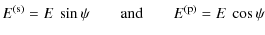
![$\displaystyle \vec{E} = E\ \left[\frac{1}{\sin \beta}\ \vec{u_{p}} - \frac{\cos \beta}{\sin \beta}\ \vec{u_{k}}\right]$](/articles/aa/full_html/2010/11/aa13906-09/img148.png)
With Eqs. (A.7) and (A.8), we find
A.2 Radiant intensity in an infinite medium
The next equations show how to obtain the intensity from the electric field amplitude. We can linked the electric field to the irradiance that is the incident power of electromagnetic radiation at a surface, per unit area.
where
Radiant intensity (incident power per unit solid angle) I and irradiance created by the electric dipole ![]() are normalized as
are normalized as
where r is the radius of the sphere where the irradiance is calculated, and
| = | |||
| = | 
|
(A.12) |
| |
and |
The normalization Eq. (A.11) let us obtain factor F:
|
|||

|
|||
![$\displaystyle \frac{P(\lambda)}{F} = \sin^{2}\theta \bigg[-\cos \alpha \bigg]_{...](/articles/aa/full_html/2010/11/aa13906-09/img173.png)
|
|||
|
|||
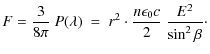
|
The radiant intensity emitted by one electric dipole
| |
(A.13) |
Consider now a luminescent layer of thickness H, and thus an ensemble of incoherently radiating electric dipoles having equal dipole moment
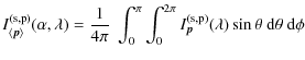
|
|||
The dipoles are located in the layer of thickness H; the total intensity emitted from this luminescent layer is thus obtained by integrating the product of
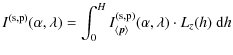
|
|||
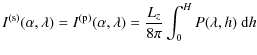
|
|||
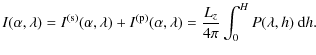
|
Let us consider now an absorbing medium with an index
- on the wave amplitude E:
E' = 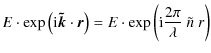
E' = 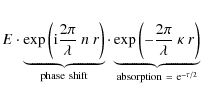
- on the wave intensity I:
I' 

I' = 
Appendix B: Effects of the interfaces of the film
In this appendix, we introduce the effects of the interfaces of the film and calculate the emission amplitude in a medium 1 by summing all the transmitted components (of each polarization), taking the phase shift and absorption due to propagation in each medium into account. As a result, the radiation pattern are obtained: it is the angular distribution of the light emitted by the film into the half-space 1.
Until now, we have considered an infinite medium. We now
consider three different homogenous media (medium 0 is a film between
semi-infinite media 1 and 2) and their interfaces. The
emitting dipole ![]() is now located in the film 0. Our aim is to determine the radiation transmitted in medium 1 under the angle of observation
is now located in the film 0. Our aim is to determine the radiation transmitted in medium 1 under the angle of observation ![]() .
.
We separate the light transmitted in medium 1 into two beams: the
direct beam D is the one emitted directly in the direction of
medium 1 (with an emission angle
![]() given by the angle of observation
given by the angle of observation
![]() and the Snell-Descartes relation of refraction). The reflected beam R
is the beam that is first directed toward medium 2 and reflected off
the interface 0/2 before being transmitted in medium 1. Each of these
beams is reflected multiple times between each interface of the
film 0. In this paragraph, we see that interference effects appear
because of these multiple reflections and also because of the sum of
the two different beams, D and R. This latter case of interference is known as the wide-angle effect.
and the Snell-Descartes relation of refraction). The reflected beam R
is the beam that is first directed toward medium 2 and reflected off
the interface 0/2 before being transmitted in medium 1. Each of these
beams is reflected multiple times between each interface of the
film 0. In this paragraph, we see that interference effects appear
because of these multiple reflections and also because of the sum of
the two different beams, D and R. This latter case of interference is known as the wide-angle effect.
![\begin{figure}
\par\includegraphics[width=12cm,clip]{13906fgB1}
\end{figure}](/articles/aa/full_html/2010/11/aa13906-09/img196.png)
|
Figure B.1:
Schematic diagram of the emission geometry for a dipole embedded in a
thin film (medium 0), at a distance h from the surface, for an emission
angle
|
| Open with DEXTER | |
B.1 The direct beam D
We first consider the the direct beam D, with its multiple reflection back and forth in layer 0, transmitted in medium 1 as shown in Fig. B.2:
|
|
= | 
|
|
![$\displaystyle \times \left[1 + \left(r_{01}^{\rm (s,p)} \ r_{02}^{\rm (s,p)} \ ...
...n \alpha_{1} \big)}_{\rm external\ phase\ shift} \right) + (...)^2 + ...\right]$](/articles/aa/full_html/2010/11/aa13906-09/img201.png)
|
|
|
= | (B.1) | |
![$\displaystyle \times \left[ 1 + \sum_{l=1}^\infty \left( r_{01}^{\rm (s,p)}\ r_...
...\tau_{0}(H) \big)\ \exp \big({\rm i}\ \delta_{1}(H) \big)\ \right)^{l} \right].$](/articles/aa/full_html/2010/11/aa13906-09/img203.png)
|
The following notations are used to lighten expressions.
Remark: ![]() is defined with a factor
is defined with a factor
![]() to obtain a power attenuation of
to obtain a power attenuation of
![]() .
.
| absorption: | |||
| phase shift: | |||
|
|||
where
Hence, one derives
|
(B.2) | ||
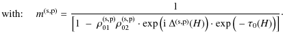
|
![\begin{figure}
\par\includegraphics[width=12cm,clip]{13906fgB2}
\end{figure}](/articles/aa/full_html/2010/11/aa13906-09/img217.png)
|
Figure B.2: Schematic diagram of the emission geometry for the direct beam D. |
| Open with DEXTER | |
B.2 The reflected beam R
![\begin{figure}
\par\includegraphics[width=12cm,clip]{13906fgB3}
\vspace*{7mm}
\end{figure}](/articles/aa/full_html/2010/11/aa13906-09/img218.png)
|
Figure B.3: Schematic diagram of the emission geometry of the reflected beam R. |
| Open with DEXTER | |
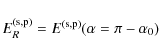
|
|
= | 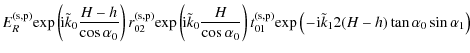
|
|
![$\displaystyle \times \left[1 + \left(r_{01}^{\rm (s,p)} \ r_{02}^{\rm (s,p)} \ ...
...{k}_{1} 2H \tan \alpha_{0} \sin \alpha_{1} \big) \right) + (...)^2 + ...\right]$](/articles/aa/full_html/2010/11/aa13906-09/img222.png)
|
|||
| = | |||
| = | 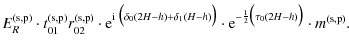
|
(B.3) |
B.3 Combination of the D and R beams
We calculated the expression of the electric field amplitude transmitted in medium 1 of the direct beam
![]() and of the reflected beam
and of the reflected beam
![]() ,
for each polarization, (s) and (p). These amplitudes are exprimed as a function of
,
for each polarization, (s) and (p). These amplitudes are exprimed as a function of
![]() and
and
![]() ,
which are the electric field amplitude emitted by an electric dipole in the direction
,
which are the electric field amplitude emitted by an electric dipole in the direction
![]() and
and
![]() ,
respectively:
,
respectively:
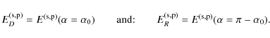
The Eqs. (A.9) and (A.10) give the influence of the angle
| (B.4) | |||
| (B.5) | |||
| (B.6) | |||
To combine the electric fields in medium 1 due to the direct and reflected beams
Let us consider the direction of the vectors
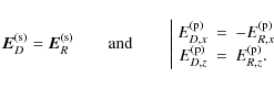
The reflection at the interface 0/2 of the reflected beam changes the sign of
- in the same direction for the s-polarization
- in opposite direction for the p-polarization.
| and: |
|
|
= | ||
![$\displaystyle \left. \pm_{(p)}^{\rm (s)} \ E_{R}^{\rm (s,p)} \cdot r_{02}^{\rm ...
...ta_{1}(H-h)\big)\big] \cdot \exp \big[- \frac{1}{2} \tau_{0}(2H-h)\big] \right]$](/articles/aa/full_html/2010/11/aa13906-09/img254.png)
|
|||
| = | (B.7) |
where
B.3.1 s-polarized
| (B.8) | |||
B.3.2 p-polarized
| (B.9) |
B.4 Radiation pattern
The radiation pattern is the angular distribution of the light emitted by the source ![]() located in layer 0 into the half-space 1, expressed by
located in layer 0 into the half-space 1, expressed by
![]() the intensity (
the intensity (
![]() )
emitted in the direction given the angles
)
emitted in the direction given the angles
![]() into the half-space 1.
into the half-space 1.
| |
= | 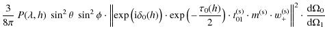
|
|
| = | (B.10) |
| |
= | ||
| = | (B.11) | ||
![$\displaystyle \times \left[\cos^{2} \theta\ \sin^{2} \alpha_{0}\ \left\Vert w_{...
...frac{1}{2} \sin{ 2 \theta} \cos \phi \sin{2 \alpha_{0}}\ w_{0}^{\rm (p)}\right]$](/articles/aa/full_html/2010/11/aa13906-09/img274.png)
|
where:
B.4.1 Solid angle modification at the interface
The ratio
![]() represents the modification of solid angle when the medium changes,
represents the modification of solid angle when the medium changes,
![]() is the radiated power in medium i into the solid angle
is the radiated power in medium i into the solid angle
![]() .
When the wave goes through the interface i/j, the solid angle is modified and the power conservation is given by Eq. (B.12) (when the transmission coefficient is 1):
.
When the wave goes through the interface i/j, the solid angle is modified and the power conservation is given by Eq. (B.12) (when the transmission coefficient is 1):
This is the origin of the factor
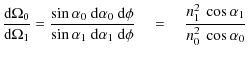
|
(B.12) |
using the derivative of the Snell-Descartes law.
B.4.2 Random orientation of the dipoles
To take a random orientation for the electric dipoles embedded in the film account, the intensity is averaged over ![]() and
and ![]() .
The geometry is thus no more dependent on the angle
.
The geometry is thus no more dependent on the angle ![]() ;
I1 is now only depending on the angle of observation
;
I1 is now only depending on the angle of observation ![]() .
.
![]() ,
which is the total power emitted in all directions of the space, at the wavelength
,
which is the total power emitted in all directions of the space, at the wavelength ![]() ,
by a single dipole
,
by a single dipole ![]() at the depth h, does not vary with the direction of the dipole.
at the depth h, does not vary with the direction of the dipole.
The intensity (
![]() )
emitted by a film layer of thickness dh, at the film depth h, is
)
emitted by a film layer of thickness dh, at the film depth h, is
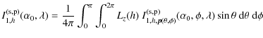
|
|||

|
|||
![$\displaystyle I_{1,h}^{\rm (s)}(\alpha_0, \lambda) = \frac{3}{32\pi^2}\ L_z(h)\...
...ht]_{0}^{\pi} \ \left[\frac{\phi}{2} - \frac{\sin (2\phi)}{4}\right]_{0}^{2\pi}$](/articles/aa/full_html/2010/11/aa13906-09/img286.png)
|
|||
| (B.13) |
| |
= | 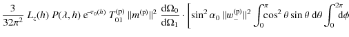
|
|
![$\displaystyle \left. + \cos^{2} \alpha_{0}\ \Vert w_{+}^{\rm (p)} \Vert^{2}\!\!...
...\theta\ {\rm d}\theta \int_{0}^{2\pi}\!\!\!\!\! \cos \phi \ {\rm d}\phi \right]$](/articles/aa/full_html/2010/11/aa13906-09/img290.png)
|
|||
| = | ![$\displaystyle \frac{3}{32\pi^2}\ L_z(h)\ P(\lambda, h)\ {\rm e}^{\!-\! \tau_{0}...
...+ \cos^{2} \alpha_{0}\ \Vert w_{+}^{\rm (p)} \Vert^{2}\ \frac{4}{3}\ \pi\right]$](/articles/aa/full_html/2010/11/aa13906-09/img291.png)
|
||
| = | (B.14) |
Finally, the specific radiant intensity in medium 1 and created by electric dipoles of random orientation at the film depth h is
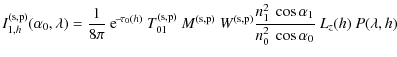
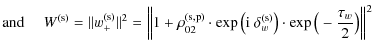
where
B.4.3 Radiant intensity observed in medium 1
Until now, we have not being interested in the wavelength dependence of the emission. The observed intensity depends on ![]() because each dipole radiates with a power
because each dipole radiates with a power
![]() that depends on the wavelength through an emission profile
that depends on the wavelength through an emission profile
![]() (in nm-1)
proper to the material of the film. In the case of photoluminescence,
the emission of each dipole will also result in an excitation absorbed
by the film (
(in nm-1)
proper to the material of the film. In the case of photoluminescence,
the emission of each dipole will also result in an excitation absorbed
by the film (
![]() is the power absorbed in unit of length (W.m-1)) that can depend on the film depth h. The emission also results in the photoluminescence yield
is the power absorbed in unit of length (W.m-1)) that can depend on the film depth h. The emission also results in the photoluminescence yield
![]()
![]() .
.
The specific power emitted by unit of film length (W nm-1 m-1) is
| (B.16) |
The total power (W) between the wavelengths
| |
= | 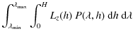
|
(B.17) |
| = | 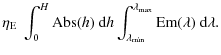
|
(B.18) |
Moreover, because the whole film is radiating, the electric dipoles
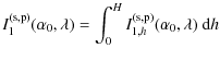
|
(B.19) | ||
| (B.20) |
The total power between the wavelengths
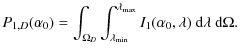
|
(B.21) |
Appendix C: Fresnel coefficients
In this appendix, we express the Fresnel coefficients for an absorbing medium (meaning with a complex refractive index).
C.1 Reflection
The Fresnel reflection coefficients are given by the equations:
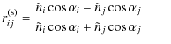
|
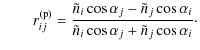
|
(C.1) |
The angles
| (C.2) |
The variables
C.2 Transmission
The Fresnel transmission coefficients (ratio of wave amplitudes) are given by the equations:

|
(C.3) |
| (C.4) |
The Fresnel transmittances (ratio of powers) are given by the equations
| |
= | 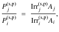
|
(C.5) |
where Ai,j is the surface section of the light beam in medium i or j, and Pi,j and
| |
= | 
|
(C.6) |
| = | (C.7) |
Remark: In the same way, the reflectance is also defined as
| (C.8) |
We can also define another transmission factor
| |
= | (C.9) | |
| = | 
|
(C.10) | |
| = | 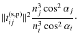
|
(C.11) |
Footnotes
- ... emission
- Appendices are only available in electronic form at http://www.aanda.org
- ... Godard
- Part of the equipment used in this work has been financed by the French INSU-CNRS program, the Physique et Chimie du Milieu Interstellaire (PCMI). This research has made use of NASA's Astrophysics Data System.
- ...

- This quartile flux width
is the difference between the third and first quartiles of the band flux (as defined by Witt & Boroson 1990). Note that
is much lower than the full width at half maximum (FWHM). In the case of a Gaussian shape:
 .
.
- ... normalized
-
 .
.
- ... superscripts
- We consider that the emission in the film is equally split up
into the two polarizations. Radiant intensities polarized s
and p emitted in the film are
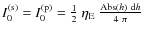 .
.
- ...%
- The variation between quantum and energetic yields is more important for PL occurring at longest wavelengths.
- ... yield
- What we call the apparent or external yield is the one obtained when not taking the optical effects of the sample geometry and measurement configuration into account.
- ...
- The adjective specific means that the variable is in unit of wavelength.
- ... total
- The contribution of polarizations (s) and (p) summed.
- ...

- The photoluminescence yield is here the energy (or power) ratio, not the quantum yield that is a photon number ratio.
All Tables
Table 1: a-C:H vibrational assignments.
Table A.1: Definition of axis, angles, and other notations.
All Figures
|
|
Figure 1: Examples of transmission spectra in the UV-visible (left) and IR region (right) of a typically produced a-C:H film. |
| Open with DEXTER | |
| In the text | |
|
|
Figure 2:
Refractive index of different a-C:H samples as a function of the optical gap (obtained by Bubenzer et al. 1983; Bourée et al. 1998; Choi 2001; Silva et al. 1996; Furton et al. 1999; Lazar 1998; Wagner & Lautenschlager 1986; Dischler et al. 1983; and Kassavetis et al. 2007). For data in red, only the
|
| Open with DEXTER | |
| In the text | |
|
|
Figure 3: sp2 fraction of different a-C:H samples as a function of the Tauc optical gap (obtained by Robertson 1996; Kleber 1991; Jarman et al. 1986; Tamor & Vassell 1994; and Kassavetis et al. 2007). The colored area corresponds to the Dartois et al. (2005) a-C:H sample (see text for details). Extreme cases of glassy carbon (Robertson 1986; Turlo & Rozwadowskajasniewska 1987), graphite (all sp2) (filled squares), and diamond (all sp3) (filled diamond) are also represented. The dashed line is a second-degree polynomial fit to these data. |
| Open with DEXTER | |
| In the text | |
|
|
Figure 4: BGO absolute PL quantum yield for different excitation wavelengths, determined by two independent methods: with a front surface device (crosses) or with an integrating sphere (circles). The variation with excitation of PL intensity (i.e. relative efficiencies) found in Weber & Monchamp (1973) is also displayed for comparison (solid line). |
| Open with DEXTER | |
| In the text | |
|
|
Figure 5:
Examples of the photoluminescence spectra of an a-C:H sample, for different excitation wavelengths (
|
| Open with DEXTER | |
| In the text | |
|
|
Figure 6:
Variation in the a-C:H photoluminescence color with the material optical gap
|
| Open with DEXTER | |
| In the text | |
|
|
Figure 7:
Variation in the a-C:H absolute photoluminescence quantum yield |
| Open with DEXTER | |
| In the text | |
|
|
Figure 8:
Variation in the a-C:H absolute photoluminescence quantum yield |
| Open with DEXTER | |
| In the text | |
|
|
Figure 9:
Variation in the a-C:H photoluminescence quantum yield |
| Open with DEXTER | |
| In the text | |
|
|
Figure 10:
Variation in the a-C:H photoluminescence band width |
| Open with DEXTER | |
| In the text | |
|
|
Figure 11:
Variation in the a-C:H photoluminescence central wavelength with the
excitation wavelength for different a-C:H samples, represented with
different colors and symbols linked by lines as guides for the eye. The
dashed line represents the equation
|
| Open with DEXTER | |
| In the text | |
|
|
Figure 12: Variation in the a-C:H photoluminescence yield with the excitation wavelength for different a-C:H samples, represented with different colors and symbols linked by lines as guides for the eye. |
| Open with DEXTER | |
| In the text | |
|
|
Figure 13:
Comparison between spectral characteristics (band width and central
wavelength) of ERE (red filled squares) and a-C:H PL (black
filled circles for our measurements and blue other symbols for a-C:H
PL data coming from previous studies (Watanabe et al. 1982; Rusli et al. 1996; Ledoux et al. 2001; Dartois et al. 2005; Lin & Feldman 1982; Xu et al. 1993; Wagner & Lautenschlager 1986; Lin & Feldman 1983; Chernyshov et al. 1991)). The ERE observations data come from Fig. 1 in Darbon et al. (1999), and we add the ERE observations corresponding to the DISM (Szomoru & Guhathakurta 1998) (square with both |
| Open with DEXTER | |
| In the text | |
|
|
Figure 14:
Comparison between quantum yield |
| Open with DEXTER | |
| In the text | |
|
|
Figure A.1:
Coordinate system and angles used to calculate the decomposition of the electric field |
| Open with DEXTER | |
| In the text | |
|
|
Figure B.1:
Schematic diagram of the emission geometry for a dipole embedded in a
thin film (medium 0), at a distance h from the surface, for an emission
angle
|
| Open with DEXTER | |
| In the text | |
|
|
Figure B.2: Schematic diagram of the emission geometry for the direct beam D. |
| Open with DEXTER | |
| In the text | |
|
|
Figure B.3: Schematic diagram of the emission geometry of the reflected beam R. |
| Open with DEXTER | |
| In the text | |
Copyright ESO 2010
Current usage metrics show cumulative count of Article Views (full-text article views including HTML views, PDF and ePub downloads, according to the available data) and Abstracts Views on Vision4Press platform.
Data correspond to usage on the plateform after 2015. The current usage metrics is available 48-96 hours after online publication and is updated daily on week days.
Initial download of the metrics may take a while.