| Issue |
A&A
Volume 515, June 2010
|
|
|---|---|---|
| Article Number | A40 | |
| Number of page(s) | 19 | |
| Section | Extragalactic astronomy | |
| DOI | https://doi.org/10.1051/0004-6361/200913871 | |
| Published online | 08 June 2010 | |
The first IRAM/PdBI polarimetric millimeter survey of active galactic nuclei
I. Global properties of the sample![[*]](/icons/foot_motif.png) ,
,
S. Trippe - R. Neri - M. Krips - A. Castro-Carrizo - M. Bremer - V. Piétu - A. L. Fontana
Institut de Radioastronomie Millimétrique (IRAM), 300 rue de la Piscine, 38406 Saint-Martin d'Hères, France
Received 14 December 2009 / Accepted 15 March 2010
Abstract
We have studied the linear polarization of 86 active galactic
nuclei (AGN) in the observed frequency range 80-267 GHz
(3.7-1.1 mm in wavelength), corresponding to rest-frame
frequencies 82-738 GHz, with the IRAM Plateau de Bure
Interferometer (PdBI). The large number of measurements, 441,
makes our analysis the largest polarimetric AGN survey in this
frequency range to date. We extracted polarization parameters via earth
rotation polarimetry with unprecedented median precisions of ![]() 0.1% in polarization fractions and
0.1% in polarization fractions and ![]() 1.2
1.2![]() in polarization angles. For 73 of 86 sources we detect
polarization at least once. The degrees of polarization are as high as
in polarization angles. For 73 of 86 sources we detect
polarization at least once. The degrees of polarization are as high as ![]() 19%, with the median over all sources being
19%, with the median over all sources being ![]() 4%. Source fluxes and polarizations are typically highly variable, with fractional variabilities up to
4%. Source fluxes and polarizations are typically highly variable, with fractional variabilities up to ![]() 60%.
We find that BLLac sources have on average the highest level of
polarization. There appears to be no correlation between degree of
polarization and redshift, indicating that there has been no
substantial change of polarization properties since
60%.
We find that BLLac sources have on average the highest level of
polarization. There appears to be no correlation between degree of
polarization and redshift, indicating that there has been no
substantial change of polarization properties since
![]() .
Our polarization and spectral index distributions are in good agreement
with results found from various samples observed at cm/radio
wavelengths; thus our frequency range is likely tracing the signature
of synchrotron radiation without noticeable contributions from other
emission mechanisms. The ``millimeter-break'' located at frequencies
.
Our polarization and spectral index distributions are in good agreement
with results found from various samples observed at cm/radio
wavelengths; thus our frequency range is likely tracing the signature
of synchrotron radiation without noticeable contributions from other
emission mechanisms. The ``millimeter-break'' located at frequencies ![]() 1 THz appears to be not detectable in the frequency range covered by our survey.
1 THz appears to be not detectable in the frequency range covered by our survey.
Key words: galaxies: active - quasars: general - polarization - techniques: polarimetric - surveys
1 Introduction
Active galactic nuclei (AGN) have been studied extensively in the wavelength range from cm-radio to ![]() radiation in the last decades (see, e.g., Kembhavi & Narlikar 1999, or Krolik 1999,
and references therein for a review). There is overwhelming
observational evidence that the main source of their emission is
accretion onto supermassive black holes (SMBH) with masses
radiation in the last decades (see, e.g., Kembhavi & Narlikar 1999, or Krolik 1999,
and references therein for a review). There is overwhelming
observational evidence that the main source of their emission is
accretion onto supermassive black holes (SMBH) with masses
![]() (e.g., Ferrarese & Ford 2005,
and references therein). However, the properties of AGN at millimeter
wavelengths are comparatively poorly known. Studies covering
substantial (more than about ten) numbers of targets in this wavelength
range mainly aim at fluxes or morphologies (e.g. Steppe
et al. 1988,1992,1993; Teräsranta et al. 1998; Sadler et al. 2008; Hardcastle & Looney 2008).
(e.g., Ferrarese & Ford 2005,
and references therein). However, the properties of AGN at millimeter
wavelengths are comparatively poorly known. Studies covering
substantial (more than about ten) numbers of targets in this wavelength
range mainly aim at fluxes or morphologies (e.g. Steppe
et al. 1988,1992,1993; Teräsranta et al. 1998; Sadler et al. 2008; Hardcastle & Looney 2008).
The linear polarization of AGN contains important information on the physics of galactic nuclei. Polarization fractions and angles provide details on synchrotron emission, the geometry of emission regions, strength and orientation of magnetic fields, and (via Faraday rotation and/or depolarization) on particle densities and matter distributions of the surrounding or outflowing matter (see, e.g., Saikia & Salter 1988, and references therein). This makes a detailed overview on the polarization properties of AGN in the millimeter wavelength range highly valuable. However, existing studies are usually limited to few selected sources (e.g. Hobbs et al. 1978; Rudnick et al. 1978; Stevens et al. 1996,1998; Attridge 2001), the work of Nartallo et al. (1998), which covers 26 sources, being a notable exception. One might also count similar studies of the black hole in the center of the Milky Way, Sgr A* (e.g. Marrone et al. 2006), and other local low-luminosity AGN (LLAGN; e.g. Bower et al. 2002) in this context.
Even if sources are not resolved spatially, polarimetric analyses provide decisive information in combination with high-resolution maps (e.g. Very Long Baseline Interferometry). One example is the relation between position angles of AGN jets and polarization angles (e.g. Stevens et al. 1996,1998; Nartallo et al. 1998). Those studies are able to constrain the magnetic field configurations in the jets and from this the types and geometries of shocks propagating through the jets.
Knowledge on the millimeter polarization of AGN is also important for technical reasons. All coherent receiver systems are sensitive to polarization by construction (see, e.g., Rohlfs & Wilson 2006, and references therein for an overview). As AGN are commonly used for flux or amplitude calibration of radioastronomical data, a non-recognized polarization of their fluxes can introduce systematic calibration errors. Therefore the construction of a polarimetric AGN catalog is helpful for improving the quality of (millimeter) radioastronomical data. Additionally, such a catalog is needful for the calibration of polarimetric observations.
Like other radioastronomical observatories, the IRAM Plateau de Bure interferometer (PdBI) uses AGN as phase and amplitude calibrators. We have used this fact to conduct a polarimetric survey of 86 sources observed from January 2007 to December 2009. The scope of this survey is to provide for the first time an overview on the polarimetric properties of AGN in the mm/radio domain based on a large number of targets. We intend to present our results in two papers: the present Paper I provides a global overview on the survey, its methods and database, presents the results derived from analyses of the sample as whole, and puts the results into the context of AGN properties at cm/radio wavelengths. Paper II is going to provide a deep analysis of a few AGN from our sample for which multiple (more than ten), time- and frequency-resolved measurements are at hand - i.e. sources for which a statistical and time series analysis per object appears promising.
2 Observations and analysis
2.1 Earth rotation polarimetry
![\begin{figure}
\par\includegraphics[angle=-90,width=8.4cm,clip]{13871f01a.eps}\h...
...e*{4mm}
\includegraphics[angle=-90,width=8.4cm,clip]{13871f01d.eps}
\end{figure}](/articles/aa/full_html/2010/07/aa13871-09/img36.png)
|
Figure 1: A polarimetric analysis
of the quasar 1642+690 as observed on May 3, 2009, at
103 GHz under good atmospheric conditions. This diagram
illustrates our data and our analysis scheme using the results from one
antenna as example. Analogous analyses are carried out for the other
five antennas. We show here V ( top left), H ( top right), (V+H) ( bottom left), and
|
| Open with DEXTER | |
In January 2007 (January 2008 for the 2 mm-band), the
antennas of the IRAM Plateau de Bure Interferometer (PdBI) were
equipped with dual linear polarization Cassegrain focus receivers.
Since then, it is possible to observe both orthogonal
polarizations - ``horizontal'' (H) and ``vertical'' (V)
with respect to the antenna frame - simultaneously. Observations
can be carried out non-simultaneous in three atmospheric windows
located around wavelengths of 1.3 mm, 2 mm,
and 3 mm. Each of these bands covers a continuous range of
frequencies; these ranges are
201-267 GHz for the 1.3 mm band, 129-174 GHz for the
2 mm band, and 80-116 GHz for the 3 mm band. Within a
given band, any frequency is available for observations (Winters &
Neri 2008)![]() .
.
The PdBI is not (yet) equipped for observations of all Stokes
parameters. We collect linear polarization data on point sources via
earth rotation polarimetry, i.e. we monitor the fluxes in the H and V channels as functions of parallactic angle ![]() .
Initially, all data (
.
Initially, all data (![]() ,
, ![]() )
are recorded as function of hour angle h (i.e. H(h), V(h)). Before calculating polarization parameters, we therefore convert hour angles h into parallactic angles
)
are recorded as function of hour angle h (i.e. H(h), V(h)). Before calculating polarization parameters, we therefore convert hour angles h into parallactic angles ![]() via
via
with l being the observatory latitude (for the PdBI,
For assessing the polarization of a source, we calculate the parameter
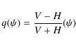
from the fluxes
This means that
For each PdBI project, we calculate ![]() before performing a flux or amplitude calibration; this allows
estimating the linear polarization of calibrator sources before using
them for this purpose. As
before performing a flux or amplitude calibration; this allows
estimating the linear polarization of calibrator sources before using
them for this purpose. As ![]() is a relative parameter, the gain factors in numerator and
denominator cancel out, meaning that a correct evaluation of
is a relative parameter, the gain factors in numerator and
denominator cancel out, meaning that a correct evaluation of ![]() does not require a gain or flux calibration. This also means that a polarization analysis using
does not require a gain or flux calibration. This also means that a polarization analysis using ![]() as parameter is not limited in accuracy by these calibration steps.
as parameter is not limited in accuracy by these calibration steps.
Due to the nature of polarized light and the fact that the
PdBI antenna receivers are located in the Cassegrain foci,
observing a polarized target results in ![]() being a cosinusoidal signal with a period of
being a cosinusoidal signal with a period of
![]() .
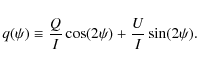
The functional form of
.
The functional form of ![]() is thus
is thus
Here mL is the fraction of linear polarization (ranging from 0 to 1; in the following, we will express mL in units of %),
For each dataset, we calculate mL, ![]() ,
and o
by means of a least-squares fit. This calculation is antenna-based,
i.e. executed for each antenna separately. The final result is the
average of the N (
,
and o
by means of a least-squares fit. This calculation is antenna-based,
i.e. executed for each antenna separately. The final result is the
average of the N (![]() )
individual antenna results. Statistical errors are standard errors
)
individual antenna results. Statistical errors are standard errors
![]() with
with ![]() being the standard deviation of parameter X over all antennas. We show an example for our analysis scheme in Fig. 1.
being the standard deviation of parameter X over all antennas. We show an example for our analysis scheme in Fig. 1.
As one can see from Eq. (4), reliably extracting polarization parameters requires a proper sampling and coverage in ![]() .
We therefore accepted only measurements which (a) cover at least 4.5 h in hour angle; (b) cover at least
.
We therefore accepted only measurements which (a) cover at least 4.5 h in hour angle; (b) cover at least
![]() (i.e.
(i.e. ![]() )
in parallactic angle; and (c) are sampled with at least five
observations per hour. A minimum angle coverage of
)
in parallactic angle; and (c) are sampled with at least five
observations per hour. A minimum angle coverage of
![]() turned out to be a good choice as it covers a large enough part of the
turned out to be a good choice as it covers a large enough part of the ![]() curve
to prevent the appearence of ambiguous solutions even in noisy data.
Using the two redundant criteria (a) and (b) is necessary
because of the behaviour of the parallactic angle for targets with
declinations
curve
to prevent the appearence of ambiguous solutions even in noisy data.
Using the two redundant criteria (a) and (b) is necessary
because of the behaviour of the parallactic angle for targets with
declinations ![]() approximately equal or larger than the observatory latitude l; this we illustrate in Fig. 2. If
approximately equal or larger than the observatory latitude l; this we illustrate in Fig. 2. If
![]() ,
the
,
the ![]() curve becomes discontinuous at transit. In those cases we use the coverage in
curve becomes discontinuous at transit. In those cases we use the coverage in ![]() (i.e. the absolute value of
(i.e. the absolute value of ![]() )
as selection criterion. If
)
as selection criterion. If
![]() and
and
![]() ,
the
,
the ![]() coverage
is continuous at transit but the angle swings quickly (within
about 1 h) from large negative to large positive values;
relying on the
coverage
is continuous at transit but the angle swings quickly (within
about 1 h) from large negative to large positive values;
relying on the ![]() coverage
alone can thus lead to a poor sampling around the transit.
Criterion (a) ensures that in any case a reasonable minimum number
of data points (>10) is included into the analysis, thus
granting a sufficient sampling.
coverage
alone can thus lead to a poor sampling around the transit.
Criterion (a) ensures that in any case a reasonable minimum number
of data points (>10) is included into the analysis, thus
granting a sufficient sampling.
In order to stabilize the model fitting, we iteratively
rejected outlier data points with unusually strong (>33% w.r.t.
the median) gain variations (caused, e.g., by unrecognized antenna
shadowing) or strong (>0.1 w.r.t. the best fit) deviation
(e.g. due to unrecognized technical problems) from the ![]() curve.
curve.
2.2 Selection of targets
Our targets are PdBI calibration sources. During each standard
PdBI observation, one or two (spatially not resolved) AGN are
monitored in parallel to the primary science target(s) for the purpose
of phase and amplitude calibration. The AGN observations are thus
a by-product of the standard interferometer operation; this makes
it possible to conduct a large AGN survey without the need for
dedicated observing time. Each calibrator is observed every ![]() 20 min for
20 min for ![]() 2 min
(usually 3 scans of 45 s each) per observation.
A typical PdBI observation lasts for several hours (
2 min
(usually 3 scans of 45 s each) per observation.
A typical PdBI observation lasts for several hours (![]() 4-8 h per science target), resulting in a corresponding number of calibrator measurements and coverage in
4-8 h per science target), resulting in a corresponding number of calibrator measurements and coverage in ![]() .
.
The selection of PdBI calibrators is based on the surveys by Steppe et al. (1988,1992,1993), Patnaik et al. (1992), Browne et al. (1998), and Wilkinson et al. (1998).
The principal selection criterion is the flux density at 90 GHz
which should be higher than 0.3 Jy. Due to source flux
variability, this cutoff is actually a soft limit. Our list of
potential targets thus includes all known mm/radio sources with minimum
flux densities ![]() 0.2 Jy at 90 GHz. Another constraint is the latidude of the PdBI (
0.2 Jy at 90 GHz. Another constraint is the latidude of the PdBI (
![]() )
which excludes reasonable observations of targets with declinations
)
which excludes reasonable observations of targets with declinations ![]()
![]()
![]() .
.
An AGN is actually observed if it can serve as a calibrator for a primary PdBI target. Therefore our sample is statistically incomplete; there is a bias towards bright sources located close to primary PdBI targets proposed by the astronomical community. This is important when comparing our results to other studies: on the one hand, our survey does not permit straightforward conclusions on physical parameters related to spatial distributions or luminosity functions of AGN samples. On the other hand, our method does not (at least not explicitly) impose a selection with respect to linear polarization, redshift, or spectral properties. Those parameters are therefore available for analysis.
2.3 Systematic uncertainties
We discuss the statistical accuracies of our analysis results in Sect. 3.1. Identifying possible systematic errors is less straightforward. As given in Eq. (2), ![]() is
a relative parameter and therefore not affected by inaccuracies of flux
or gain calibrations. However, this holds only for the case that
the gains (efficiencies) of the channels H and V are identical. Systematic gain differences may occur for the following reasons:
is
a relative parameter and therefore not affected by inaccuracies of flux
or gain calibrations. However, this holds only for the case that
the gains (efficiencies) of the channels H and V are identical. Systematic gain differences may occur for the following reasons:
- The two channels have intrinsically different sensitivities or efficiencies on timescales of a few hours or longer. Another possibility is a pointing offset on sky between the two channels. However, these properties were tested during the commissioning of the PdBI dual polarization receivers; their contribution was considered to be negligible (the IRAM commissioning team, priv. comm.).
- Instrumental polarization which is fixed with respect to the antenna frame. This effect we indeed may expect for the PdBI antennas as the receivers are located in the Cassegrain foci; this means that the entire optical system is aligned along the optical axis without rotating elements. Instrumental polarization would thus express itself as channel efficiencies that are different for the two polarizations, but do not vary with time or parallactic angle.
![\begin{figure}
\par\includegraphics[angle=-90,width=8.5cm,clip]{13871f02.eps}
\vspace*{5mm}
\end{figure}](/articles/aa/full_html/2010/07/aa13871-09/img61.png)
|
Figure 2:
Parallactic angle |
| Open with DEXTER | |
Although the influence of instrumental polarization is most probably
negligible - as long as it is not a function of h or ![]() -
we quantified the receiver polarization via a dedicated laboratory
experiment. For this we made use of a spare receiver based at the
IRAM headquarters in Grenoble (France); this receiver is
identical to the ones mounted at the PdBI antennas. The receiver
is exposed to an artificial radio signal which is perfectly linearly
polarized by using a wire grid polariser. We compare recorded signal
and emitted radiation in order to derive the instrumental polarization
of the receiver system. With our laboratory setup we are able to test
the frequency range 84-116 GHz. For this range we find receiver
polarizations of
-
we quantified the receiver polarization via a dedicated laboratory
experiment. For this we made use of a spare receiver based at the
IRAM headquarters in Grenoble (France); this receiver is
identical to the ones mounted at the PdBI antennas. The receiver
is exposed to an artificial radio signal which is perfectly linearly
polarized by using a wire grid polariser. We compare recorded signal
and emitted radiation in order to derive the instrumental polarization
of the receiver system. With our laboratory setup we are able to test
the frequency range 84-116 GHz. For this range we find receiver
polarizations of ![]() 0.3%.
We thus can conclude that the influence of instrumental polarization
(at least the component intrinsic to the receiver system) is
indeed negligible for our study.
0.3%.
We thus can conclude that the influence of instrumental polarization
(at least the component intrinsic to the receiver system) is
indeed negligible for our study.
In order to assess the global systematic uncertainty of our
analysis, we use the lowest reliable (i.e. resulting from
measurements passing all automatic quality checks plus inspection
by eye) 3![]() upper limits sm on mL from our survey as references. The corresponding figures are
upper limits sm on mL from our survey as references. The corresponding figures are
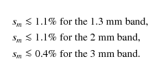
The true values are probably smaller for two reasons: (a) observations at higher frequencies suffer from lower signal-to noise ratios (S/N) in general, resulting in higher upper limits on mL; and (b) low-number statistics. Both effects seem to affect the results we quote above: the numbers for the 1.3 mm and 2 mm bands are clearly larger than the one for the 3 mm band. First, higher frequencies approximately correspond to higher upper limits as expected from effect (a). Second, we actually find for the 2 mm band about the same value as for the 1.3 mm band - as expected from effect (b) given that both samples are quite small (36 measurements each). We thus assume that the limits we quote here are actually conservative estimates - but that these are the numbers we have to use as long as additional information is not available.
3 Results
3.1 Data and accuracies
We included all PdBI calibration source data obtained from January 2007 to December 2009 into our analysis. Using the procedure and selection criteria outlined in Sect. 2, we collected 441 polarization measurements for 86 AGN, resolved in time and frequency. Our analysis covers the observed frequency range 80-267 GHz (3.7-1.1 mm in wavelength). For reasons of consistent bookkeeping, we use for all sources the epoch B1950 nomenclature throughout this article; in Table 2 we give commonly used alternative names for the most important targets. We present an overview over all observations in Table 2.
For 78 out of our 86 AGN, redshifts z are available from the literature. We collected these figures from the NASA/IPAC Extragalactic Database (NED)![]() and the MOJAVE Survey Data Archive
and the MOJAVE Survey Data Archive![]() (Lister et al. 2009).
These data are a mix of photometric and spectroscopic redshifts with
varying accuracies; in any case, the accuracies are good
enough for our purpose. Our AGN sample spans a wide range in
redshift, from z=0.02 (0316+413 = 3C 84) to z=2.69 (0239+108) with the peak of the distribution located at
(Lister et al. 2009).
These data are a mix of photometric and spectroscopic redshifts with
varying accuracies; in any case, the accuracies are good
enough for our purpose. Our AGN sample spans a wide range in
redshift, from z=0.02 (0316+413 = 3C 84) to z=2.69 (0239+108) with the peak of the distribution located at
![]() .
This means that our survey covers a rest-frame
frequency range of 82-738 GHz (as far as known). We
present the distribution of redshifts in Fig. 3.
.
This means that our survey covers a rest-frame
frequency range of 82-738 GHz (as far as known). We
present the distribution of redshifts in Fig. 3.
Thanks to the high sensitivity of the PdBI and the fact that ![]() is a relative parameter, our survey is highly precise. The median statistical errors
is a relative parameter, our survey is highly precise. The median statistical errors ![]() in mL and
in mL and ![]() are
are
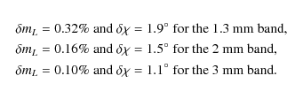
These numbers reveal a level of precision that is unprecedented (compare, e.g., Stevens et al. 1996; Nartallo et al. 1998); they also show a tendency towards higher precision for lower frequencies. We present the error distributions in Fig. 4; for reasons of visibility, we do not separate frequency bands here but show one global distribution for
![\begin{figure}
\par\includegraphics[angle=-90,width=8.5cm,clip]{13871f03.eps}
\end{figure}](/articles/aa/full_html/2010/07/aa13871-09/img66.png)
|
Figure 3: The redshift distribution of our AGN sample. For 78 out of our 86 sources redshifts z are available from the literature. Our sample covers redshifts from 0.02 to 2.69. |
| Open with DEXTER | |
![\begin{figure}
\par\includegraphics[angle=-90,width=8.5cm,clip]{13871f04a.eps}\par\includegraphics[angle=-90,width=8.5cm,clip]{13871f04b.eps}
\end{figure}](/articles/aa/full_html/2010/07/aa13871-09/img67.png)
|
Figure 4:
Distributions of statistical errors in polarization fraction
|
| Open with DEXTER | |
3.2 Polarization levels
We actually detected polarization in 316 (out of 441)
measurements; the remaining 125 were non-detections resulting
in polarization fraction upper limits. Out of our 86 AGN, we
found for 73 of them significant polarization at least once;
the remaining 13 objects remained unpolarized (within errors)
during our monitoring campaign. For 45 sources we detect
polarization at least twice; for seven sources, the number of
positive measurements exceeds ten. This corresponds to high detection
rates: for ![]() 72% of all measurements (
72% of all measurements (![]() 85%
of all sources) we actually see polarized emission. The polarization
fractions we find range from 0.6% (1928+738 at 93.2 GHz in
November 2009) to 19.4% (1005+066 at 83.3 GHz in
January 2008) with a median of
85%
of all sources) we actually see polarized emission. The polarization
fractions we find range from 0.6% (1928+738 at 93.2 GHz in
November 2009) to 19.4% (1005+066 at 83.3 GHz in
January 2008) with a median of ![]() 4.1%. In Fig. 5
we present two histograms of polarization fractions: one including all
measurements (top panel), one including one averaged (in time
and frequency) value per source (center and bottom panel).
The histograms are shown together with the best-fitting Poissonian
profiles (generalized to non-integer bin values).
4.1%. In Fig. 5
we present two histograms of polarization fractions: one including all
measurements (top panel), one including one averaged (in time
and frequency) value per source (center and bottom panel).
The histograms are shown together with the best-fitting Poissonian
profiles (generalized to non-integer bin values).
![\begin{figure}
\par\includegraphics[angle=-90,width=8.8cm,clip]{13871f05a.eps}\p...
...eps}\par\includegraphics[angle=-90,width=8.8cm,clip]{13871f05c.eps}
\end{figure}](/articles/aa/full_html/2010/07/aa13871-09/img68.png)
|
Figure 5:
Histograms of fractional linear polarization. Top panel: all measurements which detected linear polarization. Center panel: one averaged (over both times and frequencies) value per source. Bottom panel: same as center panel,
but separating the contributions of different source types.
Errorbars are binomial errors. The black curves indicate the
best-fitting Poissonian profiles; the corresponding
|
| Open with DEXTER | |
The distribution of source-averaged polarization fractions (Fig. 5, center panel) can roughly be described by a Poissonian distribution; a goodness-of-fit test finds
![]() = 1.51 (d.o.f. being the number of degrees of freedom), meaning a probability of
= 1.51 (d.o.f. being the number of degrees of freedom), meaning a probability of ![]() 10% that the distribution is indeed intrinsically Poissonian. For the distribution of all measurements (Fig. 5, top panel) we find
10% that the distribution is indeed intrinsically Poissonian. For the distribution of all measurements (Fig. 5, top panel) we find
![]() = 3.20,
meaning a probability of agreement of less than 0.1%. This is
a priori not surprising as this histogram includes multiple
measurements of sources (
= 3.20,
meaning a probability of agreement of less than 0.1%. This is
a priori not surprising as this histogram includes multiple
measurements of sources (![]() 4 in
average), i.e. correlated data. However, in both histograms
there is a marginal trend towards a pronounced tail (maybe even
bimodality) of the distributions. This may indicate a systematic
difference between source types.
4 in
average), i.e. correlated data. However, in both histograms
there is a marginal trend towards a pronounced tail (maybe even
bimodality) of the distributions. This may indicate a systematic
difference between source types.
In order to investigate this quantitatively, we grouped our sources into Seyfert galaxies, BL Lacertae (BLLac) objects, and QSOs (the last group including sources of unknown type or unclear classification). Like the redshifts, we took the source classifications from the NED and the MOJAVE archive. From all 73 AGN with detected polarization, 24 are of type BLLac, 10 are Seyfert galaxies, and 39 are QSOs/unclear. The average degrees of polarization are
Errors are standard errors
3.3 Polarization vs. frequency
![\begin{figure}
\par\includegraphics[angle=-90,width=8.8cm,clip]{13871f06a.eps}\par\includegraphics[angle=-90,width=8.8cm,clip]{13871f06b.eps}
\end{figure}](/articles/aa/full_html/2010/07/aa13871-09/img71.png)
|
Figure 6:
Top panel: degree of linear polarization vs. observed
frequency. The three groups of data points correspond to the
1.3 mm, 2 mm, and 3 mm bands of the PdBI. There is
no clear correlation between frequency and polarization fraction; in
each band, the data are approximately confined to the same range of
values. The grey-shaded area marks the ``sensitivity floor'' where no
data are available due to S/N constraints. Bottom panel: degree of linear polarization vs. rest-frame frequency. This diagram includes only sorces for which a redshift is known. The Pearson coefficient
|
| Open with DEXTER | |
As our dataset spans approximately a factor three in observed frequencies ![]() and a factor nine in rest-frame frequencies
and a factor nine in rest-frame frequencies ![]() ,
one needs to take into account possible correlations between polarization parameters and frequency. In Fig. 6
we present all polarization fraction measurements as function of
observed (top panel) and rest-frame (bottom panel) frequency. When
testing for the presence of a trend in the distribution, one needs to
be cautious for two reasons. First, the dataset includes multiple
measurements of sources at different frequencies, meaning there are
correlations among the data points. Second, there is a bias towards
higher values for mL at higher observed
frequencies due to data quality: measurements at higher observed
frequencies tend towards lower S/N (see Sect. 3.1), thus
reducing the probability for detecting small mL values (i.e. increasing the incompleteness for small mL). In the top panel of Fig. 6
this becomes visible as a ``sensitivity floor'' that rises linearly
towards larger frequencies. For interpreting the relation between
polarization and observed frequency, we therefore choose a careful
approach and only take into account the ranges the data points occupy
in the
,
one needs to take into account possible correlations between polarization parameters and frequency. In Fig. 6
we present all polarization fraction measurements as function of
observed (top panel) and rest-frame (bottom panel) frequency. When
testing for the presence of a trend in the distribution, one needs to
be cautious for two reasons. First, the dataset includes multiple
measurements of sources at different frequencies, meaning there are
correlations among the data points. Second, there is a bias towards
higher values for mL at higher observed
frequencies due to data quality: measurements at higher observed
frequencies tend towards lower S/N (see Sect. 3.1), thus
reducing the probability for detecting small mL values (i.e. increasing the incompleteness for small mL). In the top panel of Fig. 6
this becomes visible as a ``sensitivity floor'' that rises linearly
towards larger frequencies. For interpreting the relation between
polarization and observed frequency, we therefore choose a careful
approach and only take into account the ranges the data points occupy
in the ![]() diagram. One finds that in each wavelength band the data are approximately confined to the same range of values.
diagram. One finds that in each wavelength band the data are approximately confined to the same range of values.
Multiple measurements of the same source provide additional
information. As mentioned in Sect. 3.2, we have seven
sources at hand for which polarization was detected more than ten
times. When inspecting the polarizations as function of frequency,
it turns out that the only relevant effect is variability with
time. On the one hand, degrees of polarizations tend to scatter by
several per cent (i.e., by factors up to ![]() 2)
even if measured at the same frequency. On the other hand,
polarization levels measured at different frequencies are always
located around the same typical value, i.e. the data are in
agreement with flat lines in
2)
even if measured at the same frequency. On the other hand,
polarization levels measured at different frequencies are always
located around the same typical value, i.e. the data are in
agreement with flat lines in ![]() diagrams
(or they just form point clouds). We will discuss the behaviour of
individual sources in detail in Paper II.
diagrams
(or they just form point clouds). We will discuss the behaviour of
individual sources in detail in Paper II.
When inspecting the relation between polarization and rest-frame frequency (Fig. 6,
bottom panel) there is no indication for a correlation either. We
quantify the presence (or absence) of a correlation by using the
Pearson correlation coefficient ![]() (e.g. Snedecor & Cochran 1980). For the
(e.g. Snedecor & Cochran 1980). For the ![]() distribution, we find
distribution, we find
![]() ;
this indicates the absence of an intrinsic correlation. Again, one
has to take into account that this distribution contains multiple
measurements of sources, meaning the data are not fully independent.
;
this indicates the absence of an intrinsic correlation. Again, one
has to take into account that this distribution contains multiple
measurements of sources, meaning the data are not fully independent.
From our discussion we therefore conclude that (within our uncertainties) there is no indication for a correlation between frequency and degree of polarization in our data.
3.4 Polarization vs. redshift
![\begin{figure}
\par\includegraphics[angle=-90,width=8.8cm,clip]{13871f07.eps}
\end{figure}](/articles/aa/full_html/2010/07/aa13871-09/img77.png)
|
Figure 7: Distribution of mean
linear polarization fraction vs. source redshift. The diagram includes
all sources with known redshift that have been observed to be polarized
at least once; this is the case for 65 AGN. For each source
one polarization value averaged over time and frequency is shown.
According to their classification, sources are labeled as Seyfert
galaxy, BLLac object, or QSO/unclear (``QSO/?''). The Pearson
coefficient
|
| Open with DEXTER | |
For 65 out of our 86 AGN, we have detected polarization at least once and have redshift information at hand. In Fig. 7 we present the distribution of source-averaged polarization fractions
![]() vs. source redshifts z. We additionally grouped our sources into Seyfert galaxies, BLLac objects, and QSOs/unclear. From visual inspection of the
vs. source redshifts z. We additionally grouped our sources into Seyfert galaxies, BLLac objects, and QSOs/unclear. From visual inspection of the
![]() diagram, there appears to be no obvious patter in the distribution. For the distribution shown in Fig. 7, we find a Pearson correlation coefficient
diagram, there appears to be no obvious patter in the distribution. For the distribution shown in Fig. 7, we find a Pearson correlation coefficient
![]() ,
clearly indicating the absence of a correlation between redshift and
degree of polarization. We note that the maximum redshift of Seyfert
galaxies in our sample is z=1.4, well below the maximum redshifts of the other source types.
,
clearly indicating the absence of a correlation between redshift and
degree of polarization. We note that the maximum redshift of Seyfert
galaxies in our sample is z=1.4, well below the maximum redshifts of the other source types.
3.5 Polarization vs. spectral index
Combining our polarization data with flux information can provide
valuable physical information. For this study we make use of flux data
from the PdBI calibrator flux monitoring program (Krips
et al., in prep.). As for many sources the
PdBI flux monitoring provides frequency-resolved flux density
information, we computed spectral indices where possible. For this we
made use of the standard assumption that the flux density ![]() is related to the frequency
is related to the frequency ![]() via a power law
via a power law
![]() with
with ![]() being the spectral index.
being the spectral index.
Our analysis is complicated by two effects: (a) it is not possible
to observe several frequencies simultaneously with the PdBI, meaning we
have to use non-simultaneous flux data; (b) our targets show
strong intrinsic variabilities up to ![]() 60% (fractional standard deviation) at any given frequency. These effects mean that the
60% (fractional standard deviation) at any given frequency. These effects mean that the
![]() relations
we analyze show a lot of scatter which prevents us from testing models
more complicated than simple power laws (like, e.g., spectral
turnovers, or broken power laws). Within these limitations, we
have not found a case for which the simple power law model is not
sufficient for describing the data.
relations
we analyze show a lot of scatter which prevents us from testing models
more complicated than simple power laws (like, e.g., spectral
turnovers, or broken power laws). Within these limitations, we
have not found a case for which the simple power law model is not
sufficient for describing the data.
We computed ![]() by means of a least-squares fit. We performed the calculation for those
55 sources for which at least seven measurements (because the
measurements are non-simultaneous) covering a frequency range of
50 GHz or more (in order to ensure a reasonable accuracy of
the slope) are available. The substantial scatter in the
by means of a least-squares fit. We performed the calculation for those
55 sources for which at least seven measurements (because the
measurements are non-simultaneous) covering a frequency range of
50 GHz or more (in order to ensure a reasonable accuracy of
the slope) are available. The substantial scatter in the ![]() data leads to quite large formal statistical errors
data leads to quite large formal statistical errors
![]() .
We find a median uncertainty of 0.19, with the largest value being
.
We find a median uncertainty of 0.19, with the largest value being
![]() .
.
![\begin{figure}
\par\includegraphics[angle=-90,width=8.8cm,clip]{13871f08.eps}
\end{figure}](/articles/aa/full_html/2010/07/aa13871-09/img84.png)
|
Figure 8:
Histogram of spectral indices |
| Open with DEXTER | |
In Fig. 8 we present a histogram of the spectral indices. The distribution covers a range in ![]() from -0.2 to +1.3. The median spectral index is located at
from -0.2 to +1.3. The median spectral index is located at
![]() .
This shows that our sample is composed of sources with spectra that are
preferentially flat or of moderate steepness. In order to test a
potential relation between spectral index and polarization properties,
we inspected the source-averaged polarization fraction
.
This shows that our sample is composed of sources with spectra that are
preferentially flat or of moderate steepness. In order to test a
potential relation between spectral index and polarization properties,
we inspected the source-averaged polarization fraction
![]() as function of
as function of ![]() .
The corresponding diagram is presented in Fig. 9. We find a Pearson correlation coeficient
.
The corresponding diagram is presented in Fig. 9. We find a Pearson correlation coeficient
![]() ;
this indicates that there is no strict correlation between spectral
index and polarization fraction. However, this value points out a
trend towards sources with lower
;
this indicates that there is no strict correlation between spectral
index and polarization fraction. However, this value points out a
trend towards sources with lower ![]() having larger polarization fractions. This is actually visible by eye: for
having larger polarization fractions. This is actually visible by eye: for
![]() ,
the data span a range in polarization fractions up to
,
the data span a range in polarization fractions up to ![]() 12.5%; for
12.5%; for
![]() ,
there are no data beyond
,
there are no data beyond
![]() %.
We do not see a relation between source class (Seyfert, BLLac, QSO) and
location in the diagram (except of the - already discussed -
fact that BLLac objects tend to be those with the highest
polarization).
%.
We do not see a relation between source class (Seyfert, BLLac, QSO) and
location in the diagram (except of the - already discussed -
fact that BLLac objects tend to be those with the highest
polarization).
![\begin{figure}
\par\includegraphics[angle=-90,width=8.8cm,clip]{13871f09.eps}
\vspace*{5mm}
\end{figure}](/articles/aa/full_html/2010/07/aa13871-09/img89.png)
|
Figure 9:
Source-averaged degree of linear polarization
|
| Open with DEXTER | |
We summarize our survey in Table 1.
For each source we give B1950 name, redshift, spectral indices and
their uncertainties, fluxes and flux variabilities, polarization
fractions and their variabilities, and polarization angles and their
variabilities as far as available. According to their frequencies,
measurements are grouped into 1.3 mm, 2 mm, and 3 mm
wavelength bands. Please note that we quote source variabilities ![]() ;
these values are standard deviations over measurements from different dates. These are not
accuracies of individual measurements, which are usually much smaller
than the intrinsic variabilities (cf. Sect. 3.1 and Fig. 4).
Entries ``-'' denote ``not observed''. If a source was
observed but no polarization could be detected, we quote the 3-
;
these values are standard deviations over measurements from different dates. These are not
accuracies of individual measurements, which are usually much smaller
than the intrinsic variabilities (cf. Sect. 3.1 and Fig. 4).
Entries ``-'' denote ``not observed''. If a source was
observed but no polarization could be detected, we quote the 3-![]() upper limit on mL; those values are denoted by ``<''.
upper limit on mL; those values are denoted by ``<''.
Table 1: Fluxes and polarization parameters for our sample of 86 AGN.
4 Discussion
Our survey provides an overview over the polarimetric properties of
AGN at millimeter wavelengths. In order to put our results into
context, one needs to take into account that our source sample is
biased with respect to brightness. As our targets serve as
calibrators, there is a preferential selection of bright AGN located
close to primary PdBI targets. Our sources are mm/radio-bright (
![]() Jy at 3 mm; see Table 1)
and have (as far as known) spectra that are consistent with power
law spectra. We therefore assume in the following that the emission we
observe is fully non-thermal.
Jy at 3 mm; see Table 1)
and have (as far as known) spectra that are consistent with power
law spectra. We therefore assume in the following that the emission we
observe is fully non-thermal.
For synchrotron emission from an ensemble of homogeneous and
isotropic relativistic electrons moving in a uniform magnetic field
(B-field), the degree of linear polarization can be calculated
analytically. If the energy distribution of the electrons follows
a power law with index ![]() ,
then
,
then
![]() and
and

(e.g. Pacholczyk 1970) for optically thin sources. For flat-spectrum sources with
(e.g. Pacholczyk 1970). For
The distribution of the source-averaged polarization fractions (see Fig. 5) provides two conclusions. First, we do see a trend that BLLac sources have higher intrinsic polarization levels. Second, there is no obvious segregation of source types; the distributions show a large amount of overlap, indicating a smooth transition between source types.
The absence of a correlation between redshift and (source-averaged) degree of polarization (see Fig. 7) provides interesting constraints on the time evolution of AGN. As we observe polarized emission in 65 sources with ![]() ,
our sample probes a substantial part of the age of the universe.
From this we can conclude that the properties of polarized mm radiation
from AGN have not evolved substantially since
,
our sample probes a substantial part of the age of the universe.
From this we can conclude that the properties of polarized mm radiation
from AGN have not evolved substantially since
![]() .
.
The spectral indices of our sources are located in the range
![]() (see Fig. 8). This indicates that our sample actually provides a mix of core-dominated (
(see Fig. 8). This indicates that our sample actually provides a mix of core-dominated (
![]() )
and outflow (lobe/jet)-dominated (
)
and outflow (lobe/jet)-dominated (
![]() ;
e.g. Krolik 1999)
sources. On the one hand, the absence of a clear correlation between
spectral index and degree of polarization (see Fig. 9)
suggests that (at least at mm wavelengths) the polarization
levels of AGN cores and outflows are of the same order of
magnitude. On the other hand, there is a marginal trend towards
higher polarization in core-dominated sources; this leaves room for
systematically higher polarization levels in AGN cores compared to
outflows by factors
;
e.g. Krolik 1999)
sources. On the one hand, the absence of a clear correlation between
spectral index and degree of polarization (see Fig. 9)
suggests that (at least at mm wavelengths) the polarization
levels of AGN cores and outflows are of the same order of
magnitude. On the other hand, there is a marginal trend towards
higher polarization in core-dominated sources; this leaves room for
systematically higher polarization levels in AGN cores compared to
outflows by factors ![]() 2.
2.
Our results are in good agreement with AGN properties observed in the
centimeter wavelength range, with respect to the distributions of
polarization fractions and spectral indices obtained from various
samples. The surveys by Altschuler & Wardle (1976,1977) and Aller et al. (1985) found maximum polarizations of ![]() 15% in the frequency range 2-14.5 GHz, with ``typical'' degrees of polarization being
15% in the frequency range 2-14.5 GHz, with ``typical'' degrees of polarization being ![]() 5%.
This is especially interesting as our survey probes the high-frequency
end of the ``pure synchrotron'' domain of the AGN spectral energy
distribution. At frequencies above
5%.
This is especially interesting as our survey probes the high-frequency
end of the ``pure synchrotron'' domain of the AGN spectral energy
distribution. At frequencies above ![]() 1 THz,
other radiation processes like Compton scattering in the accretion zone
around the central black hole can contribute substantially to the
emission (e.g. Krolik 1999, and references therein). Observationally, this transition expresses itself in the ``millimeter-break'' located at
1 THz,
other radiation processes like Compton scattering in the accretion zone
around the central black hole can contribute substantially to the
emission (e.g. Krolik 1999, and references therein). Observationally, this transition expresses itself in the ``millimeter-break'' located at ![]() THz (e.g. Elvis et al. 1994).
We find for our frequency range the same characteristic radiation
properties - in terms of polarization and distribution of
spectral indices - as for the cm wavelength range. From
this we can conclude that the rest-frame frequency range up to
738 GHz traces - like the cm/radio continuum domain -
the signatures of ``pure'' synchrotron emission without noticeable
contributions from other emission mechanisms. The mm-break appears to
be not detectable in the frequency range covered by our survey.
A one-to-one comparison of results for given sources across
various studies is beyond the scope of this article. However, we are
going to discuss individual sources and corresponding multi-wavelegth
observations in detail in Paper II.
THz (e.g. Elvis et al. 1994).
We find for our frequency range the same characteristic radiation
properties - in terms of polarization and distribution of
spectral indices - as for the cm wavelength range. From
this we can conclude that the rest-frame frequency range up to
738 GHz traces - like the cm/radio continuum domain -
the signatures of ``pure'' synchrotron emission without noticeable
contributions from other emission mechanisms. The mm-break appears to
be not detectable in the frequency range covered by our survey.
A one-to-one comparison of results for given sources across
various studies is beyond the scope of this article. However, we are
going to discuss individual sources and corresponding multi-wavelegth
observations in detail in Paper II.
We find that substantial variations in the degree of polarization (up to ![]() 60%
in fractional standard deviation) on timescales from weeks to years are
a common feature throughout our AGN sample (see Table 1). This is the case also for the source fluxes that show variabilities at a similar level.
60%
in fractional standard deviation) on timescales from weeks to years are
a common feature throughout our AGN sample (see Table 1). This is the case also for the source fluxes that show variabilities at a similar level.
Any discussion of variability in polarization is clearly limited by the
sparse and irregular sampling (both in time and frequency) of our
polarization data (see also Sect. 3.2). However,
in flux, variability on various time scales is a well-known
feature and has been explored in long-term studies, notably the works
by Hovatta et al. (2007,2008)
that cover time lines of 25 years. From a detailed statistical
analysis they conclude that (a) characteristic time scales for
variations are ![]() 1
to 6 years depending on the strengths of the variations;
(b) variations are the more seldom the stronger they are;
(c) there is a characteristic flare length of
1
to 6 years depending on the strengths of the variations;
(b) variations are the more seldom the stronger they are;
(c) there is a characteristic flare length of ![]() 2.5 years;
and (d) source variability and characteristic time scales are not
related to source type (QSO, BLLac, galaxy).
2.5 years;
and (d) source variability and characteristic time scales are not
related to source type (QSO, BLLac, galaxy).
From this we can conclude that (1) the variability we observe in polarization levels fits the present picture of AGN variability; but that (2) our survey probably has not yet reached the time coverage to be sensitive to the characteristic time scales of variations which have been seen in light curves. It is interesting to note that Hovatta et al. (2007,2008) find no relation between flux variability and source type, whereas we find a relation between polarization level and source type (see Sect. 3.2). It will therefore be important to test for the presence of a relation between polarization variability and source type as soon as this becomes feasible. We are going to discuss this in Paper II which deals with sources for which we have multiple (>10) polarization measurements at hand.
High variabilities in both, fluxes and polarization fractions, point towards strong variations in source activities, accretion flows, B-field geometries, and/or outflows (jets) on the timescales of our survey. The most common explanation of such violent behaviour are shocks occuring in relativistic jets, possibly accompanied by jet bending and changes in B-field configurations (e.g. Stevens et al. 1998; Nartallo et al. 1998). Other, more recent models propose the orbital motion of plasma concentrations (``hotspots'') in the accretion disks of supermassive black holes in order to explain flux and polarization variations on timescales from hours to weeks (e.g. Broderick & Loeb 2006). In any case, our results indicate that these processes are a frequent phenomenon for luminous AGN.
5 Summary and conclusions
We have made use of IRAM/PdBI calibration measurements in order to
collect polarimetric data for 86 active galactic nuclei in the observed frequency range 80-267 GHz, corresponding to a rest-frame
frequency range 82-738 GHz. We obtain 441 measurements in
total and find significant linear polarization in 316 measurements
belonging to 73 sources. Our survey achieves unprecedented precisions
with median errors of ![]() 0.1% in polarization fractions and
0.1% in polarization fractions and ![]() 1.2
1.2![]() in polarization angles. Additionally, we collect source flux data from
the PdBI calibrator monitoring. The main results are:
in polarization angles. Additionally, we collect source flux data from
the PdBI calibrator monitoring. The main results are:
- The median polarization fraction for our sources is
 4%, the highest value found is 19%. These numbers are far below the value
  60%
expected from ``ideal'' synchrotron emission from optically thin
sources, pointing towards a substantial averaging of polarization due
to limited spatial resolution and non-uniform B-field geometries, and
maybe also emission from optically thick source regions.
60%
expected from ``ideal'' synchrotron emission from optically thin
sources, pointing towards a substantial averaging of polarization due
to limited spatial resolution and non-uniform B-field geometries, and
maybe also emission from optically thick source regions.
- The source-averaged degrees of polarization follow
approximately a Poisson distribution with a slight trend towards a
pronounced tail or bimodality. In average, BLLac sources show a
larger degree of polarization (
 %) than Seyfert galaxies or QSOs (
 % and
% and
 %, respectively).
- The spectral indices of our AGN are located in the range
 to +1.3,
indicating that our sample is a mix of core- and outflow-dominated
sources. There is no clear correlation between polarization and
spectral index, but there is a trend towards higher polarization
fractions in core-dominated sources.
to +1.3,
indicating that our sample is a mix of core- and outflow-dominated
sources. There is no clear correlation between polarization and
spectral index, but there is a trend towards higher polarization
fractions in core-dominated sources.
- We do not find correlations of polarization with rest-frame frequencies (shown by a Pearson correlation coefficient
 )
or redshifts. The absence of a mL-z correlation (
)
or redshifts. The absence of a mL-z correlation (
 )
indicates that there has been no noticable change of polarization properties since
)
indicates that there has been no noticable change of polarization properties since
 .
.
- The values and distributions we find for mL and
 are
in good agreement with results obtained from various samples and
studies in the centimeter wavelength range (though we do not attempt a
one-to-one comparison of sources here). This indicates that the
rest-frame frequency range we probe (
are
in good agreement with results obtained from various samples and
studies in the centimeter wavelength range (though we do not attempt a
one-to-one comparison of sources here). This indicates that the
rest-frame frequency range we probe (
 GHz)
can be described as a continuation of the cm/radio continuum domain for
which synchrotron radiation is the only noteworthy emission mechanism.
Especially, the mm-break appears to be not detectable in our
frequency range.
GHz)
can be described as a continuation of the cm/radio continuum domain for
which synchrotron radiation is the only noteworthy emission mechanism.
Especially, the mm-break appears to be not detectable in our
frequency range.
- The high variabilities of polarization fractions and source fluxes (up to 60%)
strengthen the picture that violent processes - like shocks in
relativistic jets or plasma ``hotspots'' moving in accretion
disks - are a frequent phenomenon.
We would like to thank Jan Martin Winters (IRAM Grenoble) for his help with the treatment of PdBI data. We are grateful to Ivan Agudo (IAA Granada) and Thomas Krichbaum (MPIfR Bonn) for helpful discussions on polarimetry and AGN polarization. Our work has made use of the NASA/IPAC Extragalactic Database (NED) which is operated by the Jet Propulsion Laboratory, California Institute of Technology, under contract with the National Aeronautics and Space Administration. We have made use of data from the MOJAVE database that is maintained by the MOJAVE team (Lister et al. 2009). Last but not least, we are grateful to the reviewer, E. Ros, who helped to improve the quality of this article.
References
- Aller, H. D., Aller, M. F., Latimer, G. E., & Hodge, P. E. 1985, ApJS, 59, 513 [NASA ADS] [CrossRef] [Google Scholar]
- Altschuler, D. R., & Wardle, J. F. C. 1976, MNRAS, 82, 1 [Google Scholar]
- Altschuler, D. R., & Wardle, J. F. C. 1977, MNRAS, 179, 153 [NASA ADS] [Google Scholar]
- Attridge, J. M. 2001, ApJ, 553, L31 [NASA ADS] [CrossRef] [Google Scholar]
- Beltrán, M. T., Gueth, F., Guilloteau, S., & Dutrey, A. 2004, A&A, 416, 631 [NASA ADS] [CrossRef] [EDP Sciences] [Google Scholar]
- Bower, G. C., Falcke, H., & Mellon, R. R. 2002, ApJ, 578, L103 [NASA ADS] [CrossRef] [Google Scholar]
- Broderick, A. E., & Loeb, A. 2006, MNRAS, 367, 905 [NASA ADS] [CrossRef] [Google Scholar]
- Browne, I. W. A., Wilkinson, P. N., Patnaik, A. R., & Wrobel, J. M. 1998, MNRAS, 293, 257 [NASA ADS] [CrossRef] [Google Scholar]
- Elvis, M., Wilkes, B. J., McDowell, J. C., et al. 1994, ApJS, 95, 1 [NASA ADS] [CrossRef] [Google Scholar]
- Ferrarese, L., & Ford, H. 2005, Space Sci. Rev., 116, 523 [NASA ADS] [CrossRef] [Google Scholar]
- Hobbs, R. W., Maran, S. P., & Brown, L. W. 1978, ApJ, 223, 373 [NASA ADS] [CrossRef] [Google Scholar]
- Hovatta, T., Tornikoski, M., Lainela, M., et al. 2007, A&A, 469, 899 [NASA ADS] [CrossRef] [EDP Sciences] [Google Scholar]
- Hovatta, T., Nieppola, E., Tornikoski, M., et al. 2008, A&A, 485, 51 [NASA ADS] [CrossRef] [EDP Sciences] [Google Scholar]
- Hardcastle, M. J., & Looney, L. W. 2008, MNRAS, 388, 176 [NASA ADS] [CrossRef] [Google Scholar]
- Kembhavi, A. K., & Narlikar, J. V. 1999, Quasars and Active Galactic Nuclei (Cambridge University Press) [Google Scholar]
- Krolik, J. H. 1999, Active Galactic Nuclei (Princeton University Press) [Google Scholar]
- Lister, M. L., Aller, H. D., Aller, M. F., et al. 2009, AJ, 137, 3718 [NASA ADS] [CrossRef] [Google Scholar]
- Marrone, D. P., Moran, J. M., Zhao, J.-H., & Rao, R. 2006, ApJ, 640, 308 [NASA ADS] [CrossRef] [Google Scholar]
- Nartallo, R., Gear, W. K., Murray, A. G., Robson, E. I., & Hough, J. H. 1998, MNRAS, 297, 667 [NASA ADS] [CrossRef] [Google Scholar]
- Pacholczyk, A. G. 1970, Radio Astrophysics (Freeman) [Google Scholar]
- Patnaik, A. R., Browne, I. W. A., Wilkinson, P. N., & Wrobel, J. M. 1992, MNRAS, 254, 655 [NASA ADS] [CrossRef] [Google Scholar]
- Rohlfs, K., & Wilson, T. L. 2006, Tools of Radio Astronomy (Springer) [Google Scholar]
- Rudnick, L., Owen, F. N., Jones, T. W., Puschell, J. J., & Stein, W. A. 1978, ApJ, 225, L5 [NASA ADS] [CrossRef] [Google Scholar]
- Sadler, E. M., Ricci, R., Ekers, R. D., et al. 2008, MNRAS, 385, 1656 [NASA ADS] [CrossRef] [Google Scholar]
- Saikia, D. J., & Salter, C. J. 1988, ARA&A, 26, 93 [NASA ADS] [CrossRef] [Google Scholar]
- Sault, R. J., Hamaker, J. P., & Bregman, J. D. 1996, A&AS, 117, 149 [NASA ADS] [CrossRef] [EDP Sciences] [Google Scholar]
- Snedecor, G. W., & Cochran, W. G. 1980, Statistical Methods (Iowa State University Press) [Google Scholar]
- Steppe, H., Salter, C. J., Chini, R., et al. 1988, A&AS, 75, 317 [NASA ADS] [Google Scholar]
- Steppe, H., Liechti, S., Mauersberger, R., et al. 1992, A&AS, 96, 441 [NASA ADS] [Google Scholar]
- Steppe, H., Paubert, G., Sievers, A., et al. 1993, A&AS, 102, 611 [NASA ADS] [Google Scholar]
- Stevens, J. A., Robson, E. I., & Holland, W. S. 1996, ApJ, 462, L23 [NASA ADS] [CrossRef] [Google Scholar]
- Stevens, J. A., Robson, E. I., Gear, W. K., et al. 1998, ApJ, 502, 182 [NASA ADS] [CrossRef] [Google Scholar]
- Teräsranta, H., Tornikoski, M., Mujunen, A., et al. 1998, A&AS, 132, 305 [NASA ADS] [CrossRef] [EDP Sciences] [Google Scholar]
- Thompson, A. R., Moran, J. M., & Swenson, G. W. 2001, Interferometry and Synthesis in Radio Astronomy, 2nd edn. (Wiley-Interscience) [Google Scholar]
- Wilkinson, P. N., Browne, I. W. A., Patnaik, A. R., Wrobel, J. M., & Sorathia, B. 1998, MNRAS, 300, 790 [NASA ADS] [CrossRef] [Google Scholar]
- Winters, J. M., & Neri, R. 2008, An Introduction to the IRAM Plateau de Bure Interferometer, public IRAM document, version 4.0-10 [Google Scholar]
Online Material
Table 2: Observations journal of our AGN survey.
Footnotes
- ... sample
- This study is based on observations carried out with the IRAM Plateau de Bure Interferometer. IRAM is supported by INSU/CNRS (France), MPG (Germany), and IGN (Spain).
- ...
- Table 2 is only available in electronic form at http://www.aanda.org
- ...2008)
- http://www.iram.fr/IRAMFR/GILDAS/doc/pdf/pdbi-intro.pdf
- ... (NED)
- Accessible via http://nedwww.ipac.caltech.edu/
- ... Archive
- See http://www.physics.purdue.edu/MOJAVE/allsources.shtml
All Tables
Table 1: Fluxes and polarization parameters for our sample of 86 AGN.
Table 2: Observations journal of our AGN survey.
All Figures
|
|
Figure 1: A polarimetric analysis
of the quasar 1642+690 as observed on May 3, 2009, at
103 GHz under good atmospheric conditions. This diagram
illustrates our data and our analysis scheme using the results from one
antenna as example. Analogous analyses are carried out for the other
five antennas. We show here V ( top left), H ( top right), (V+H) ( bottom left), and
|
| Open with DEXTER | |
| In the text | |
|
|
Figure 2:
Parallactic angle |
| Open with DEXTER | |
| In the text | |
|
|
Figure 3: The redshift distribution of our AGN sample. For 78 out of our 86 sources redshifts z are available from the literature. Our sample covers redshifts from 0.02 to 2.69. |
| Open with DEXTER | |
| In the text | |
|
|
Figure 4:
Distributions of statistical errors in polarization fraction
|
| Open with DEXTER | |
| In the text | |
|
|
Figure 5:
Histograms of fractional linear polarization. Top panel: all measurements which detected linear polarization. Center panel: one averaged (over both times and frequencies) value per source. Bottom panel: same as center panel,
but separating the contributions of different source types.
Errorbars are binomial errors. The black curves indicate the
best-fitting Poissonian profiles; the corresponding
|
| Open with DEXTER | |
| In the text | |
|
|
Figure 6:
Top panel: degree of linear polarization vs. observed
frequency. The three groups of data points correspond to the
1.3 mm, 2 mm, and 3 mm bands of the PdBI. There is
no clear correlation between frequency and polarization fraction; in
each band, the data are approximately confined to the same range of
values. The grey-shaded area marks the ``sensitivity floor'' where no
data are available due to S/N constraints. Bottom panel: degree of linear polarization vs. rest-frame frequency. This diagram includes only sorces for which a redshift is known. The Pearson coefficient
|
| Open with DEXTER | |
| In the text | |
|
|
Figure 7: Distribution of mean
linear polarization fraction vs. source redshift. The diagram includes
all sources with known redshift that have been observed to be polarized
at least once; this is the case for 65 AGN. For each source
one polarization value averaged over time and frequency is shown.
According to their classification, sources are labeled as Seyfert
galaxy, BLLac object, or QSO/unclear (``QSO/?''). The Pearson
coefficient
|
| Open with DEXTER | |
| In the text | |
|
|
Figure 8:
Histogram of spectral indices |
| Open with DEXTER | |
| In the text | |
|
|
Figure 9:
Source-averaged degree of linear polarization
|
| Open with DEXTER | |
| In the text | |
Copyright ESO 2010
Current usage metrics show cumulative count of Article Views (full-text article views including HTML views, PDF and ePub downloads, according to the available data) and Abstracts Views on Vision4Press platform.
Data correspond to usage on the plateform after 2015. The current usage metrics is available 48-96 hours after online publication and is updated daily on week days.
Initial download of the metrics may take a while.