| Issue |
A&A
Volume 515, June 2010
|
|
|---|---|---|
| Article Number | A9 | |
| Number of page(s) | 12 | |
| Section | Celestial mechanics and astrometry | |
| DOI | https://doi.org/10.1051/0004-6361/200913785 | |
| Published online | 31 May 2010 | |
Accurate free and forced rotational motions of rigid Venus
L. Cottereau - J. Souchay - S. Aljbaae
Observatoire de Paris, Systèmes de Référence Temps Espace (SYRTE), CNRS/UMR8630, Paris, France
Received 1 December 2009 / Accepted 27 February 2010
Abstract
Context. The precise and accurate modelling of a
terrestrial
planet like Venus is an exciting and challenging topic, all the more
interesting because it can be compared with that of Earth for which
such a modelling has already been achieved at the milli-arcsecond
level.
Aims. We aim to complete a previous study, by
determining the
polhody at the milli-arcsecond level, i.e. the torque-free
motion
of the angular momentum axis of a rigid Venus in a body-fixed frame,
as well as the nutation of its third axis of figure in space,
which is fundamental from an observational point of view.
Methods. We use the same theoretical framework as
Kinoshita
(1977, Celest. Mech., 15, 277) did to determine the precession-nutation
motion of a rigid Earth. It is based on a representation of
the
rotation of a rigid Venus, with the help of Andoyer variables and a set
of canonical equations in Hamiltonian formalism.
Results. In a first part we computed the polhody, we
showed that
this motion is highly elliptical, with a very long period of
525 cy compared with 430 d for the Earth. This is due
to the
very small dynamical flattening of Venus in comparison with our planet.
In a second part we precisely computed the Oppolzer terms, which allow
us to represent the motion in space of the third Venus figure axis with
respect to the Venus angular momentum axis under the influence of the
solar gravitational torque. We determined the corresponding tables of
the nutation coefficients of the third figure axis both in longitude
and in obliquity due to the Sun, which are of the same order of
amplitude as for the Earth. We showed that the nutation coefficients
for the third figure axis are significantly different from those of the
angular momentum axis on the contrary of the Earth. Our analytical
results have been validated by a numerical integration, which revealed
the indirect planetary effects.
Key words: planets and satellites: individual: Venus - celestial mechanics
1 Introduction
Venus, which can be considered as the twin sister of the Earth with
regard to its global characteristics (size, mass, density), has been
the subject of a good amount of investigations on very long time scales
to understand its slow retrograde rotation (243 d) and its
rather
small obliquity (
![]() )
(Goldstein 1964;
Carpenter 1964;
Goldreich & Peale 1970;
Lago & Cazenave 1979;
Dobrovoskis 1980;
Yoder 1995;
Correia & Laskar 2001,
2003).
Habibullin (1995)
made an analytical study on the rotation of a rigid Venus. In Cottereau
& Souchay (2009)
we presented an alternative study, from a theoretical framework already
used by Kinoshita (1977)
for the rigid Earth. We made an accurate description of the motion of
rotation of Venus at short time scale. We calculated the ecliptic
coordinates of the Venus orbital pole and the reference point
)
(Goldstein 1964;
Carpenter 1964;
Goldreich & Peale 1970;
Lago & Cazenave 1979;
Dobrovoskis 1980;
Yoder 1995;
Correia & Laskar 2001,
2003).
Habibullin (1995)
made an analytical study on the rotation of a rigid Venus. In Cottereau
& Souchay (2009)
we presented an alternative study, from a theoretical framework already
used by Kinoshita (1977)
for the rigid Earth. We made an accurate description of the motion of
rotation of Venus at short time scale. We calculated the ecliptic
coordinates of the Venus orbital pole and the reference point
![]() ,
which is the equivalent of the vernal equinox for Venus. Our value for
the precession in longitude was
,
which is the equivalent of the vernal equinox for Venus. Our value for
the precession in longitude was ![]() t/cy
t/cy ![]() 66.5.
We performed a full calculation of the nutation coefficients of Venus
and presented the complete tables of nutation in longitude
66.5.
We performed a full calculation of the nutation coefficients of Venus
and presented the complete tables of nutation in longitude
![]() and obliquity
and obliquity
![]() for the angular momentum axis due to both the dynamical flattening and
triaxiality of the planet.
for the angular momentum axis due to both the dynamical flattening and
triaxiality of the planet.
In this paper, the study begun in Cottereau & Souchay (2009) is completed. First we consider in Sect. 2 the torque-free rotational motion of a rigid Venus. We recall the parametrization of Kinoshita (1977) and the important equations of Kinoshita (1972), which are used to solve this torque-free motion. The important characteristics (amplitude, period, trajectory) of the free motion are given. Cottereau & Souchay (2009) assumed that the relative angular distances between the three poles (of angular momentum, figure and rotation) are very small as is the case for the Earth. In this paper we want to accurately determine the motion of the third Venus figure axis, which is the fundamental one from an observational point of view. To do that we reject the hypothesis of coincidence of the poles. Thus we determine the Oppolzer terms depending on the dynamical flattening and the trixiality of Venus. Then we compare these terms with the corresponding nutations terms for the angular momentum axis, as determined by Cottereau & Souchay (2009) and the Oppolzer terms determined by Kinoshita (1977) for the Earth in Sect. 3. We give the complete tables of the nutation coefficients of the third figure axis of Venus. We compare them with the nutation coefficients of the angular momentum axis taken from Cottereau & Souchay (2009) (Sect. 4). Finally in Sect. 5 we determine the nutation of the angular momentum axis by numerical integration using the ephemeris DE405. We validate the analytical results of Cottereau & Souchay (2009) down to a precision of the order of a relative 10-5. We show that the discrepancies between the numerical integration and analytical results (Cottereau & Souchay 2009) are caused by the indirect planetary effect, i.e. by the small contribution to the nutation, which is due to the periodic oscillations of the orbital motion of Venus. In this paper as in Cottereau & Souchay (2009) our domain of validity is roughly 3000 years.
![\begin{figure}
\par\includegraphics[width=9cm,clip]{13785f1.eps}
\end{figure}](/articles/aa/full_html/2010/07/aa13785-09/img17.png)
|
Figure 1: Relation between the Euler angles and the Andoyer variables. |
| Open with DEXTER | |
2 Torque-free motion for rigid Venus
2.1 Equation of torque-free motion
We consider the problem of the rotational motion of the rigid Venus in
absence of any external force. We note (
0, X, Y,
Z) the inertial frame and (0,x,y,z)
the cartesian coordinates fixed to the rigid body of the planet
(see Fig. 1).
The orientation of Venus with respect to the inertial axes is
determined through the Euler angles (![]() ,
,
![]() ,
,
![]() ). The
parameter
). The
parameter ![]() gives the position of the prime meridian (0,x)
with respect to
gives the position of the prime meridian (0,x)
with respect to
![]() (Kinoshita 1977).
The angular momentum axis (hereafter denoted AMA) of Venus is the axis
directed along G. The components of the
angular momentum referred to the body-fixed axes are:
(Kinoshita 1977).
The angular momentum axis (hereafter denoted AMA) of Venus is the axis
directed along G. The components of the
angular momentum referred to the body-fixed axes are:
| (1) |
where A, B, C are the principal inertia moments of Venus. Moreover the kinetic energy is
| (2) |
To describe the torque-free rotational motion we use the Andoyer variables (Andoyer 1923; Kinoshita 1972) (see Fig. 1):
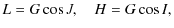
- L the angular momentum component along the 0z axis;
- H the angular momentum component along the 0Z axis;
- G the angular momentum amplitude of Venus;
- l the angle between the origin meridian Ox and the node P;
- h the longitude of the node of the AMA
with respect to
 ;
;
- g the longitude of the plane node (0, X, Y) with respect to Q and to the equatorial plane.
where I, J are the angle between the AMA and the inertial axis (O, Z) and the angle between the AMA and the third figure axis (hereafter denoted TFA) respectively. Using spherical trigonometry, we determine the following relation between the variables:
| (4) |
The components of the angular momentum vector with the Andoyer variables are
| Lz=L. | (5) |
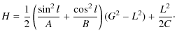
The Hamiltonien for the torque-free motion of Venus corresponding to the kinetic energy is
![\begin{figure}
\par\includegraphics[angle=-90,width=8cm,clip]{13785f2.ps}
\end{figure}](/articles/aa/full_html/2010/07/aa13785-09/img31.png)
|
Figure 2: Isoenergetic curves of Venus in the (J, l) phase space of the torque-free motion. Two motions are showen: ``the libration motion'' and the ``circulation motion''. |
| Open with DEXTER | |
The Hamiltonian H does not depend on time and is free from g and h. Thus the number of degrees of freedom of the torque-free motion is one. Deprit (1967) has characterized this motion by studying the isoenergetic curves in the phase plane L-l. But we prefer to study the isoenergetic curves in the (J, l) phase space using Eq. (3). This allows a good description of the position of the AMA with respect to the TFA. Figure 2 shows the two possible motions: one is the libration motion and the other one the circulation motion. Using the values of the relative differences of the moments of inertia of Williams (private communication)
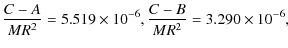
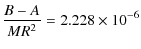
and addopting
with
and
where e measures the triaxiality of the rigid body (Andoyer 1923). Applying these formulas to Venus we get
2.2 Canonical transformations
To determine the torque-free motion of Venus, we use the method described in full detail by Kinoshita (1972). We give here only the important results and equations which are needed to apply this study to Venus. The Hamiltonian for the torque-free motion is given by Eq. (6). To solve the equations of motion, we perform a canonical transformation which replaces the angular momentum by its action variable (Goldstein 1964). First we make two intermediate transformations to simplify the computation.
2.2.1 First transformation
We change (
L, G,
l, g) to (
![]() ,
,
![]() ,
u1, u2)
using the Hamilton Jacobi method (Chazy 1953). We note
,
u1, u2)
using the Hamilton Jacobi method (Chazy 1953). We note ![]() )
the characteristic function. We have the Hamilton-Jacobi equation
)
the characteristic function. We have the Hamilton-Jacobi equation
where
|
(12) |
This equation can be solved as
where
![\begin{displaymath}%
\gamma^2=\left[2\alpha_{1}-\frac{1}{2}\left(\frac{1}{A}+\frac{1}{B}\right)\alpha_{2}^2\right]D.
\end{displaymath}](/articles/aa/full_html/2010/07/aa13785-09/img49.png)
|
(14) |
The constants e and D are given by Eqs. (9) and (10). Because the new Hamiltonian depends on only one of the momenta
|
||

|
(15) |
2.2.2 Second transformation
Then we make another transformation, which changes (
![]() ,
u1, u2)
to
,
u1, u2)
to ![]() .
The two momenta are defined as follows:
.
The two momenta are defined as follows:
With these new coordinates the Hamiltonian F0 becomes
|
(17) |
Thanks to the Hamilton equations the conjugate variables are
Using (16) we get
| (20) |
and
where j is defined in Sect. 2.1. Now we can introduce the canonical transformation, which replaces the angular momentum by its action variable.
2.2.3 Action variables
The action variables are given by:
|
||
| (22) |
where
We obtain
where
| (25) |
and
![$\displaystyle %
\wedge_{0}=\frac{2}{\pi}\Big[E(k)F(\chi,k')+K(k)E(\chi,k')-K(k)F(\chi,k')\Big],$](/articles/aa/full_html/2010/07/aa13785-09/img71.png)
with
|
(27) |
In Eq. (26) K(k) is the complete elliptic integral of the first kind with modulus
| (28) |
| (29) |
where
Here the epoch of time t is defined so that
Table 1: Important values of the free motion of Venus.
2.3 Venus free rotation
As a result we can use a development of our variables g,
l and J with respect
to j and e. The
results of these technical developments (Kinoshita 1972) are summarized
in the Appendix. As is the case for the Earth we assume that
the angle j of Venus is very small.
Table 1
gives the numerical values of the important constants used in the
theory of the free motion of Venus. To calculate these values
we
take ![]() (Yoder 1995)
and the values of the moment of inertia given in Eq. (7). The value
of D and
(Yoder 1995)
and the values of the moment of inertia given in Eq. (7). The value
of D and ![]() are unknown. Finally we find
are unknown. Finally we find
|
|||
|
|||
|
|||
![$\displaystyle \quad\;~ + ~ 2.05548 (l^{*}-\tilde{l})\biggl]\Biggl]+O(j^4)$](/articles/aa/full_html/2010/07/aa13785-09/img90.png)
|
|||
Using the developments for a small e, we get
|
||
|
||
![$\displaystyle J=\tilde{J}[1.00933+0.11154 \cos 2\tilde{l}]+O(e^3, j^2)$](/articles/aa/full_html/2010/07/aa13785-09/img95.png)
|
||
|
(32) |
Because the main limitation of our calculation is the uncertainty on the ratio
![\begin{figure}
\par\includegraphics[width=7cm,clip]{13785f3.eps}
\end{figure}](/articles/aa/full_html/2010/07/aa13785-09/img99.png)
|
Figure 3:
(X, Y)
free motion of Venus in space for five hundred century time space (red
and blue curves). The green curve represents a circle with the radius |
| Open with DEXTER | |
We note here that the value of j has been chosen arbitrarily, for it does not significantly affect the polhody, except the amplitude. We see that the torque-free motion of Venus is an elliptic motion, as is the case for the Earth. The rotational free motion of Venus, with a period Tl=525 centuries (Table 1) is much slower than that of Earth (303 d). If we consider the elastic Earth (ocean and atmosphere), the torque-free motion has a period of 432 d, significantly larger than in the rigid case. The atmosphere of Venus is much denser than that of the Earth. So it would be interesting to study the torque-free motion of the elastic Venus in a next paper.
3 Rigid Venus forced rotational motion
In Cottereau & Souchay (2009) we assumed that the relative angular distances between the three poles of Venus (pole of angular momentum, of figure and of rotation) are very small, as is the case for the Earth. In this section we determine the motion of the TFA, which is the fundamental one from an observational point of view. To do so we reject the hypothesis of coincidence of the poles. Using the spherical trigonometry in the triangle (P, Q, R) (see Fig. 1) we determine the relations between the TFA and the AMA. Supposing that the angle J between the AMA and the TFA is small we obtain
where I characterizes the obliquity and h the motion of precession-nutation in longitude of the AMA of Venus.
where
We see that Eqs. (37) and (38) are functions of
3.1 Equations of motion
The Hamiltonian related to the rotational motion of Venus is (Cottereau
& Souchay 2009)
| (39) |
where
![\begin{displaymath}%
U \!= \! \frac{\mathtt{{\vec G}} M'}{r^3}\left[\frac{2C-A-B...
...lta )+\frac{A-B}{4}P_2^{2} (\sin \delta) \cos 2\alpha \right],
\end{displaymath}](/articles/aa/full_html/2010/07/aa13785-09/img112.png)
where
In Eq.(40) we only consider the potential in first order. The method for solving the equation of motion is described in Kinoshita (1977). Only the final results are given. We have

where
![$\displaystyle +~ \frac{A-B}{4}P_{2}^{2} \sin \delta \cos 2\alpha \Bigg]{\rm d}t.$](/articles/aa/full_html/2010/07/aa13785-09/img120.png)
We use a transformation described by Kinoshita (1977) and based on the Jacobi polynomials. It expresses
![$\displaystyle -~\frac{1}{2} \sin 2I P_{2}^1(\sin \beta)\cos 2(\lambda - h)\Bigg]$](/articles/aa/full_html/2010/07/aa13785-09/img125.png)
![$\displaystyle \times ~ P_{2}^2(\sin \beta)\cos(2\lambda-2h-\epsilon g)\Bigg]+\sin^2 J$](/articles/aa/full_html/2010/07/aa13785-09/img130.png)
![$\displaystyle \times ~ \sum_{\epsilon =\pm 1}(1+\epsilon \cos I)^2P_{2}^2(\sin \beta)\cos 2(\lambda-h-\epsilon g)\Bigg].$](/articles/aa/full_html/2010/07/aa13785-09/img133.png)
and
![$\displaystyle +~ \frac{1}{8}\sin^2 IP_{2}^2(\sin \beta)\cos 2(\lambda-h-\epsilon l)\Bigg]$](/articles/aa/full_html/2010/07/aa13785-09/img137.png)
![$\displaystyle \times ~ P_{2}^2(\sin \beta)\cos(2\lambda-2h-2\rho\epsilon l-\epsilon g)\Bigg].$](/articles/aa/full_html/2010/07/aa13785-09/img143.png)
To simplify the calculations, we separately study the symmetric part of Eq. (44), which depends on the dynamical flattening, and the antisymmetric part, which depends on the triaxiality of Venus. So the dynamical flattening coefficient of will be noted with an ``s'' index and the triaxiality coefficient with an ``a'' index. From its definition above, we can set
3.2 Oppolzer terms depending on the dynamical flattening
Using Eqs. (44)
and (45)
with ![]() ,
we have
,
we have
| Ws1 | = | ![$\displaystyle \frac{\mathtt{{\vec G}} M'}{a^3}\frac{2C-A-B}{2}\int \left[\left(\frac{a}{r}\right)^3P_{2}(\sin \delta)\right]{\rm d}t$](/articles/aa/full_html/2010/07/aa13785-09/img146.png)
|
|
| = | |||
| (46) |
where
| Ws10 | = | 
|
|
![$\displaystyle \left. - ~ \frac{1}{4}\sin^2I\int\cos 2(\lambda-h)\left(\frac{a}{r}\right)^3{\rm d}t\right]$](/articles/aa/full_html/2010/07/aa13785-09/img150.png)
|
(47) |
![$\displaystyle \left. + ~\frac{1}{4}(1+\cos I)\int\cos (2\lambda-2h-g)\left(\frac{a}{r}\right)^3 {\rm d}t\right]$](/articles/aa/full_html/2010/07/aa13785-09/img153.png)
| Ws12 | = | 
|
|
![$\displaystyle \left. -~ \frac{1}{4}(1+\cos I)^2\int\cos 2(\lambda-h-g)\left(\frac{a}{r}\right)^3{\rm d}t\right],$](/articles/aa/full_html/2010/07/aa13785-09/img156.png)
|
(49) |
and
|
(50) |
According to the Hamilton equations, we obtain
|
|
= | 
|
|
![$\displaystyle \left. + ~\frac{1}{2}\cos^2 J \ W_{s12}\right]$](/articles/aa/full_html/2010/07/aa13785-09/img160.png)
|
|||
| (51) |
We assume that the angle J is small as for the Earth. This yields
![$\displaystyle \frac{1}{G}\left[-3 W_{s0}-\frac{1}{ J}W_{s11}+\frac{1}{2} W_{s12}\right]$](/articles/aa/full_html/2010/07/aa13785-09/img162.png)
We have also
![$\displaystyle \frac{1}{G}\left[\cos^2J \ \frac{\partial W_{s11}}{\partial g}-\frac{1}{8}\sin 2J \ \frac{\partial W_{s12}}{\partial g}\right]$](/articles/aa/full_html/2010/07/aa13785-09/img164.png)
Using Eqs. (52) and (53) we obtain the Oppolzer terms depending on the dynamical flattening

![$\displaystyle \frac{1}{G \sin I}\Bigg[\frac{\partial W_{s11}}{\partial g}\sin g - W_{s11} \cos g\Bigg]+O(J)$](/articles/aa/full_html/2010/07/aa13785-09/img167.png)
![$\displaystyle \frac{1}{G}\left[\frac{\partial W_{s11}}{\partial g} cos g+W_{s11} \sin g \right]+O(J).$](/articles/aa/full_html/2010/07/aa13785-09/img170.png)
To solve Eqs. (54) and (55) through Ws11 given by Eq. (48), it is necessary to develop
Table 2:
Development of ![]() of Venus. t is counted in Julian centuries.
of Venus. t is counted in Julian centuries.
Table 3:
Development of ![]() of Venus. t is counted in Julian centuries.
of Venus. t is counted in Julian centuries.
Table 4:
Development of ![]() of Venus. t is counted in Julian centuries.
of Venus. t is counted in Julian centuries.
The numerical value for Tg is given in Table 1. We recall here that our domain of validity is 3000 years as it was in Cottereau & Souchay (2009).
Table 5:
Oppolzer terms in longitude depending on dynamical flattening [
![]() :
nutation coefficients of the AMA].
:
nutation coefficients of the AMA].
Table 6:
Oppolzer terms in the obliquity depending on dynamical flattening [
![]() :
nutation coefficients of the AMA].
:
nutation coefficients of the AMA].
![\begin{figure}
\par\includegraphics[width=8cm,clip]{13785f4.eps}
\end{figure}](/articles/aa/full_html/2010/07/aa13785-09/img200.png)
|
Figure 4: Nutation of the AMA (red curve) and nutation of the Oppolzer terms (blue and bolt curve) in the obliquity of Venus depending on its dynamical flattening for a 1000 d span, from J2000.0. |
| Open with DEXTER | |
Because of the the developments above we give in Tables 5 and 6
the Oppolzer terms, in longitude and in obliquity
respectively,
depending on the dynamical flattening. For comparison we give the
corresponding nutation coefficients (in brackets) of the AMA
determined in Cottereau & Souchay (2009). They are
represented in both Figs. 4
and 5
for a 1000 d time span to see the leading
oscillations. We
remark that the Oppolzer terms are of the same order of magnitude as
the nutation coefficients. The Oppolzer terms associated with the
argument M are even larger. This is due to
the low value of ![]() rd/cy,
which enters in the denominator during the integration of the equations
of motion. Whereas for the calculation of the corresponding
AMA coefficient only the numerical value
rd/cy,
which enters in the denominator during the integration of the equations
of motion. Whereas for the calculation of the corresponding
AMA coefficient only the numerical value
![]() rd/cy
appears, which is higher than
rd/cy
appears, which is higher than
![]() .
In Figs. 4
and 5,
showing the Oppolzer terms, the presence of the sinusoid with a period
of 224 d reflects this. Remark (Table 6) that the Oppolzer
terms associated with the argument M
and 2M
have a non zero amplitude, whereas the nutation coefficients of the AMA
associated with the same arguments do not exist. Indeed we remark here
that to compute the nutation coefficients in obliquity for this axis,
we performed the derivative of W1
with respect to h, which does not appear in
the terms associated with the argument M
and 2M. Notice also that for the Earth (see
Kinoshita 1977),
the Oppolzer terms depending on the dynamical flattening are
negligible with respect to the nutation coefficients of the AMA. The
largest Oppolzer term in longitude in Kinoshita (1977) is
.
In Figs. 4
and 5,
showing the Oppolzer terms, the presence of the sinusoid with a period
of 224 d reflects this. Remark (Table 6) that the Oppolzer
terms associated with the argument M
and 2M
have a non zero amplitude, whereas the nutation coefficients of the AMA
associated with the same arguments do not exist. Indeed we remark here
that to compute the nutation coefficients in obliquity for this axis,
we performed the derivative of W1
with respect to h, which does not appear in
the terms associated with the argument M
and 2M. Notice also that for the Earth (see
Kinoshita 1977),
the Oppolzer terms depending on the dynamical flattening are
negligible with respect to the nutation coefficients of the AMA. The
largest Oppolzer term in longitude in Kinoshita (1977) is ![]() ,
whereas for Venus it is
,
whereas for Venus it is
![]() .
In obliquity it is
.
In obliquity it is
![]() ,
whereas for Venus it is
,
whereas for Venus it is
![]() .
The rapid rotation of the Earth compared with the slow retrograde
rotation of Venus explains this contrast: the frequencies,
which
depend on the rotation g and enter in the
denominator during the integration, are 104 times
higher for the Earth than for Venus.
.
The rapid rotation of the Earth compared with the slow retrograde
rotation of Venus explains this contrast: the frequencies,
which
depend on the rotation g and enter in the
denominator during the integration, are 104 times
higher for the Earth than for Venus.
![\begin{figure}
\par\includegraphics[width=8cm,clip]{13785f5.eps}
\end{figure}](/articles/aa/full_html/2010/07/aa13785-09/img208.png)
|
Figure 5: Nutation of the AMA (red curve) and nutation of the Oppolzer terms (blue and bolt curve) in longitude of Venus depending on its dynamical flattening for a 1000 d span, from J2000.0. |
| Open with DEXTER | |
Due to its slow rotation, the triaxiality of Venus (1.66 ![]() 10-6)
is not negligible compared to the dynamical flattening (1.31
10-6)
is not negligible compared to the dynamical flattening (1.31 ![]() 10-5).
Thus the Oppolzer terms depending on the triaxiality must be considered
and are calculated below.
10-5).
Thus the Oppolzer terms depending on the triaxiality must be considered
and are calculated below.
3.3 Oppolzer terms depending on the triaxiality
From Eq. (44),
we have
| Wa1 | = | ![$\displaystyle \frac{\mathtt{{\vec G}} M'}{a^3}\frac{A-B}{4}\int \left[\left(\frac{a}{r}\right)^3P_{2}^2(\sin \delta) \cos 2\alpha\right]{\rm d}t$](/articles/aa/full_html/2010/07/aa13785-09/img209.png)
|
|
| = | |||
|
(56) |
where
| Wa10 | = | 
|
|
|
|||
|
(57) |
|
|
= | 
|
|
|
|||
![$\displaystyle \left. \times ~ \int \left(\frac{a}{r}\right)^3\cos (2\lambda-2h-2\rho l-g){\rm d}t\right]$](/articles/aa/full_html/2010/07/aa13785-09/img220.png)
|
(58) |
|
|
= | 
|
|
![$\displaystyle \left. \times ~ \int \left(\frac{a}{r}\right)^3\cos 2(\lambda-h-\rho l-g){\rm d}t \right],$](/articles/aa/full_html/2010/07/aa13785-09/img225.png)
|
(59) |
and
|
(60) |
Using the Hamilton equations and assuming, as for the terms depending on the dynamical flattening, that J is a small angle, we obtain
and
![$\displaystyle - ~ \frac{1+\cos J}{G}\left[\frac{\partial W_{a11(1)}}{\partial l}-\cos J \ \frac{\partial W_{a11(1)}}{\partial g}\right]$](/articles/aa/full_html/2010/07/aa13785-09/img232.png)
![$\displaystyle +~ \frac{(1+\cos J)^2}{4G\sin J}\left[\frac{\partial W_{a12(\rho)}}{\partial l}-\cos J \ \frac{\partial W_{a12(\rho)}}{\partial g}\right]\cdot$](/articles/aa/full_html/2010/07/aa13785-09/img233.png)
As Wa11(-1) is multiplied by
|
(63) |
The Oppolzer terms depending on the triaxiality are

![$\displaystyle + ~ W_{a11(1)} \cos g\Bigg]+O(J)$](/articles/aa/full_html/2010/07/aa13785-09/img240.png)
![$\displaystyle -\frac{2}{G}\left[\frac{\partial W_{a11(1)}}{\partial g} cos g-W_{a11(1)} \sin g\right].$](/articles/aa/full_html/2010/07/aa13785-09/img243.png)
To solve Eqs. (64) and (65) it is necessary to develop
We can determine the Oppolzer terms depending on the triaxiality.
Table 7: Oppolzer terms in longitude depending on triaxiality.
Table 8: Oppolzer terms in obliquity depending on triaxiality.
Tables 7
and 8
give the Oppolzer terms in longitude and in obliquity respectively,
depending on Venus triaxiality. For comparison, we give the
corresponding nutation coefficients of the AMA determined in Cottereau
& Souchay (2009).
They are represented in both Figs. 6 and 7
for a 4000 d time span. We remark here also that the
Oppolzer
terms are more important than the corresponding nutation coefficients
of the AMA. The Oppolzer terms associated with the argument ![]() is even roughly twice larger than the corresponding nutation
coefficient. This is due to the low value of
is even roughly twice larger than the corresponding nutation
coefficient. This is due to the low value of ![]() = 944.36 rd/cy,
which appears in the denominator during the integration of the
equations of motion, whereas for the calculation of the corresponding
coefficient of the AMA only the sidereal angle frequency
= 944.36 rd/cy,
which appears in the denominator during the integration of the
equations of motion, whereas for the calculation of the corresponding
coefficient of the AMA only the sidereal angle frequency
![]() rd/cy
appears which, is significantly larger. The appearance of the
angle
rd/cy
appears which, is significantly larger. The appearance of the
angle ![]() during the integration explains that the other Oppolzer terms are more
important than the corresponding coefficient of the nutation of the
AMA, as justified in Sect. 3.2 for the
terms depending on the dynamical flattening.
during the integration explains that the other Oppolzer terms are more
important than the corresponding coefficient of the nutation of the
AMA, as justified in Sect. 3.2 for the
terms depending on the dynamical flattening.
![\begin{figure}
\par\includegraphics[width=8cm,clip]{13785f6.eps}
\end{figure}](/articles/aa/full_html/2010/07/aa13785-09/img268.png)
|
Figure 6: Nutation of the AMA (Blue and bolt curve) and nutation of the Oppolzer terms (red curve) in obliquity of Venus depending on its triaxility for a 4000 d span, from J2000.0. |
| Open with DEXTER | |
![\begin{figure}
\par\includegraphics[width=8cm,clip]{13785f7.eps}
\end{figure}](/articles/aa/full_html/2010/07/aa13785-09/img269.png)
|
Figure 7: Nutation of the AMA (Blue and bolt curve) and nutation of the Oppolzer terms (red curve) in longitude of Venus depending on its triaxility for a 4000 d span, from J2000.0. |
| Open with DEXTER | |
Other than for Earth, the Oppolzer terms in triaxiality are not negligible compared to the nominal values of the corresponding nutation coefficient. The frequencies depending on the rotation 2l+g, which enter in the denominator during the integration, are very small compared those of our planet. Now we can determine the nutation of the TFA of Venus, which is fundamental from an observational point of view.
4 Numerical results and comparison with the motion of the AMA
From Eqs. (35)
and (36)
we calculate the nutation coefficients of the TFA. We recall here that
the nutation is respectively designated in longitude by
![]() and in obliquity by
and in obliquity by
![]() .
Tables 9
and 10
give the nutation coefficients depending on the dynamical flattening in
longitude and in obliquity respectively. In a similar
way,
Tables 11
and 12
give the coefficients depending on the triaxiality.
.
Tables 9
and 10
give the nutation coefficients depending on the dynamical flattening in
longitude and in obliquity respectively. In a similar
way,
Tables 11
and 12
give the coefficients depending on the triaxiality.
Table 9:
![]() :
nutation coefficients of the TFA in longitude of Venus depending on its
dynamical flattening.
:
nutation coefficients of the TFA in longitude of Venus depending on its
dynamical flattening.
Table 10:
![]() :
nutation coefficients of the TFA in obliquity of Venus depending on its
dynamical flattening.
:
nutation coefficients of the TFA in obliquity of Venus depending on its
dynamical flattening.
Table 11:
![]() nutation coefficients of the TFA in longitude of Venus depending on its
triaxiality.
nutation coefficients of the TFA in longitude of Venus depending on its
triaxiality.
Table 12:
![]() :
nutation coefficients of the TFA in obliquity of Venus depending on its
triaxiality.
:
nutation coefficients of the TFA in obliquity of Venus depending on its
triaxiality.
In this section we will show the difference between the
nutation of the
TFA, calculated in this paper and that of the AMA of Venus (![]() and
and ![]() ),
as calculated by Cottereau & Souchay (2009).
Figures 8
and 9
represent the nutation in longitude and in obliquity of the two axes
respectively for a 4000 d time span.
),
as calculated by Cottereau & Souchay (2009).
Figures 8
and 9
represent the nutation in longitude and in obliquity of the two axes
respectively for a 4000 d time span.
Concerning the longitude we can point out two important specific remarks:
- The nutation of the TFA is significantly smaller than the nutation of the AMA. Indeed the amplitude peak to peak of the nutation of the TFA (an amplitude of 1.5'') is twice as small as that of the AMA (an amplitude of 3'').
- The nutation of the TFA is dominated by three sinusoids
associated with the arguments
 ,
M and
,
M and  ,
with respective periods 112.35 d, 224.70 d and
121.51 d
whereas the nutation of the AMA is dominated by two sinusoids of
argument
and .
,
with respective periods 112.35 d, 224.70 d and
121.51 d
whereas the nutation of the AMA is dominated by two sinusoids of
argument
and .
Finally we can highlight the differences between the Earth and
Venus. For the Earth, the nutation of the two axes (angular momentum
and third figure axis) are roughly the same (Woolard 1953; Kinoshita 1977),
whereas for Venus they are significantly different. We can also remark
that the leading nutation component of the third Venus figure axis in
longitude due to the gravitational action of the Sun, with
argument
![]() (see Eq. (9))
has an amplitude of 0
(see Eq. (9))
has an amplitude of 0
![]() 693.
This is of the same order as the leading
693.
This is of the same order as the leading
![]() the nutation amplitude of the Earth due to the Sun, i.e. 0
the nutation amplitude of the Earth due to the Sun, i.e. 0
![]() 998
despite the fact that Venus has a very small dynamical flattening.
As explained by Cottereau & Souchay (2009) this is due to
the compensating role of the very slow rotation of Venus. Moreover,
notice that for Venus the argument
998
despite the fact that Venus has a very small dynamical flattening.
As explained by Cottereau & Souchay (2009) this is due to
the compensating role of the very slow rotation of Venus. Moreover,
notice that for Venus the argument ![]() stands
for the longitude of the Sun as seen from the planet, so that
the
corresponding period of the leading nutation term with
stands
for the longitude of the Sun as seen from the planet, so that
the
corresponding period of the leading nutation term with
![]() argument
is 112.35 d, whereas it is 182.5 d for
the Earth.
argument
is 112.35 d, whereas it is 182.5 d for
the Earth.
![\begin{figure}
\par\includegraphics[width=8cm,clip]{13785f8.eps}\vspace{-2mm}
\end{figure}](/articles/aa/full_html/2010/07/aa13785-09/img274.png)
|
Figure 8: Nutation of the TFA (blue curve) and nutation of the momentum axis in longitude of Venus for 4000 d time span, from J2000.0. |
| Open with DEXTER | |
![\begin{figure}
\par\includegraphics[width=8cm,clip]{13785f9.eps}\vspace{-2mm}
\end{figure}](/articles/aa/full_html/2010/07/aa13785-09/img275.png)
|
Figure 9: Nutation of the TFA (blue curve) and nutation of the momentum axis in obliquity of Venus for 4000 d time span, from J2000.0. |
| Open with DEXTER | |
5 Determination of the indirect planetary effects on the nutation of Venus
Using the ephemeris DE405 (Standish 1998),
we computed the nutation of Venus by numerical integration with a
Runge-Kutta ![]() order
algorithm. Figures 10
and 11
show the differences between the nutations in obliquity and in
longitude of the AMA as computed from the analytical tables (Cottereau
& Souchay 2009)
and that from
the numerical integration for a 4000 d time span. The
residuals obtained clearly consist of periodic components with small
amplitudes of the order of 10-5'' in
obliquity and 10-3''
in longitude. This numerical integration validates the results
of Cottereau & Souchay (2009)
down to a relative accuracy of 10-5.
Moreover Kinoshita's model used in Cottereau & Souchay (2009)
assumed a Keplerian motion of Venus around the Sun. It is well
known that the effects of planetary attraction into Earth's orbit
(called indirect planetary effect) entails a departure from the
Keplerian motion and that this departure induces new nutation terms as
calculated by Souchay & Kinoshita (1996).
In order to infer whether the discrepancies between our numerical
integration and our analytical computation are caused by this indirect
planetary effect in Venus orbit, we performed a spectral analysis of
the residuals.
order
algorithm. Figures 10
and 11
show the differences between the nutations in obliquity and in
longitude of the AMA as computed from the analytical tables (Cottereau
& Souchay 2009)
and that from
the numerical integration for a 4000 d time span. The
residuals obtained clearly consist of periodic components with small
amplitudes of the order of 10-5'' in
obliquity and 10-3''
in longitude. This numerical integration validates the results
of Cottereau & Souchay (2009)
down to a relative accuracy of 10-5.
Moreover Kinoshita's model used in Cottereau & Souchay (2009)
assumed a Keplerian motion of Venus around the Sun. It is well
known that the effects of planetary attraction into Earth's orbit
(called indirect planetary effect) entails a departure from the
Keplerian motion and that this departure induces new nutation terms as
calculated by Souchay & Kinoshita (1996).
In order to infer whether the discrepancies between our numerical
integration and our analytical computation are caused by this indirect
planetary effect in Venus orbit, we performed a spectral analysis of
the residuals.
![\begin{figure}
\par\includegraphics[width=8cm,clip]{13785f10.eps}\vspace{-2mm}
\end{figure}](/articles/aa/full_html/2010/07/aa13785-09/img277.png)
|
Figure 10: Difference between the obliquity nutation of the AMA and the numerical integration for 4000 d time span, from J2000.0. The curve at bottom represents the residual after substracting the sinusoidal terms of Table 13. |
| Open with DEXTER | |
![\begin{figure}
\par\includegraphics[width=8cm,clip]{13785f11.eps}
\end{figure}](/articles/aa/full_html/2010/07/aa13785-09/img278.png)
|
Figure 11: Difference between the nutation in longitude of the AMA and the numerical integration for 4000 d time span, from J2000.0. The curve at bottom represents the residual after substracting the sinusoidal terms of the Table 14. |
| Open with DEXTER | |
The leading oscillations of the two signals (in longitude and in obliquity) are determined with a fast Fourier Transform (FFT). Tables 13 and 14 give the leading amplitudes and periods of the sinusoids characterizing the signal in Figs. 10 and 11, where the curve at the bottom represents the residuals after subtraction of these sinusoids. The periods presented in the Tables 13 and 14 do not correspond to any period of the tables given in the precedent section starting from the keplerian approximation. On the opposite, when comparing them with the tables of nutation of the Earth taken from Souchay & Kinoshita (1996), similar periods appear, which correspond to the combination of planetary longitudes. This is a clear confirmation that the differences between our analytical computation and our numerical integration in Figs. 10 and 11, are essentially due to the indirect planetary effects, negligible at first order and not taken previously into account by Cottereau & Souchay (2009). Tables 13 and 14 also present, when they have been clearly identified, the combination of the planetary longitudes corresponding to the detected sinusoids. We also note the corresponding amplitudes of the Earth's nutation due to the indirect effect of Venus where available. We can thus point out the similitude and reciprocity of the indirect planetary effects of Venus on the Earth rotation, and of the indirect planetary effects of the Earth on the rotation of Venus.
Table 13: Rigid Venus nutation coefficient from the indirect planetary contribution in longitude.
Table 14: Rigid Venus nutation coefficient from the indirect planetary contribution in obliquity.
6 Conclusion and prospects
We achieved the accurate study of the rotation of Venus for a rigid model and on a short time scale begun by Cottereau & Souchay (2009) by applying analytical formalisms already used for the rigid Earth (Kinoshita 1972, 1977). The differences between the rotational characteristics of Venus and our planet, due to the slow rotation of Venus and its small obliquity, have been highlighted.
Firstly we precisely determined the polhody, i.e. the torque-free rotational motion for a rigid Venus. We adopted the theory used by Kinoshita (1972, 1992) and gave the parametrization and the equations of motion to solve the motion. We showed that the polhody is significantly elliptic, quite different from the Earth, where it can be considered as circular in first approximation. Moreover it is considerably slower. Indeed, the period of the torque-free motion is 525.81 cy for Venus, whereas it is 303 d for our planet, when considered as rigid.
Then we determined the motion of the third figure axis, which is fundamental from an observational point of view. We calculated the Oppolzer terms due to the gravitational action of the Sun with the equation of motion of Kinoshita (1977) as well as the corresponding development of the disturbing functions. We compared them with the nutation coefficients for the angular momentum axis taken in Cottereau & Souchay (2009). One of the important results is that these Oppolzer terms depending on the dynamical flattening are of the same order of amplitude as the nutation coefficients themselves, whereas for the Earth (Woolard 1953; Kinoshita 1977) these Oppolzer terms are very small with respect to the nutation coefficients of the angular momentum axis. Moreover we computed the Oppolzer terms depending on the triaxiality, which is not done in Kinoshita (1977) for Earth, which they neglect. For Venus these Oppolzer terms are significant even larger than the corresponding coefficients of nutation of the angular momentum axis.
With our Oppolzer terms we were also able to give the tables
of
nutation of the third figure axis, from which we computed the nutation
for a 4000 d time span. The comparison with the
nutation of
the angular momentum axis, calculated from Cottereau & Souchay (2009),
is also given. The nutation of the third figure axis is significantly
smaller peak to peak than the nutation of the angular momentum axis in
longitude, and less important in obliquity. The amplitude of the
largest nutation coefficient in longitude of the third figure
axis (1.5'') is half that of the angular momentum
axis (3'').
The amplitude of the nutation in obliquity of the third figure axis
is 0
![]() 18
peak to peak, whereas the amplitude of the angular momentum axis
is 0
18
peak to peak, whereas the amplitude of the angular momentum axis
is 0
![]() 25.
The nutations of the third figure axis, in obliquity
and in
longitude, are dominated by three sinusoids associated with the
arguments
25.
The nutations of the third figure axis, in obliquity
and in
longitude, are dominated by three sinusoids associated with the
arguments
![]() , M
and
, M
and ![]() ,
with respective periods 112.35 d, 224.70 d and
121.51 d.
The nutation of the angular momentum axis is dominated by two sinusoids
with the argument
,
with respective periods 112.35 d, 224.70 d and
121.51 d.
The nutation of the angular momentum axis is dominated by two sinusoids
with the argument
![]() and
and ![]() .
Our results showed that although the axis of angular momentum
and
the third figure axis can be considered identical for Earth (Kinoshita 1977), this
approximation does not hold for a slowly rotating
planet Venus.
.
Our results showed that although the axis of angular momentum
and
the third figure axis can be considered identical for Earth (Kinoshita 1977), this
approximation does not hold for a slowly rotating
planet Venus.
We validated our analytical results down to a relative accuracy of 10-5 with a numerical integration. Moreover, we confirmed by using results in Souchay & Kinoshita (1996) for the nutation of a rigid Earth that the differences between our analytical computation and our numerical integration are essentially due to the indirect planetary effects, which was not taken into account by Cottereau & Souchay (2009). This study is fundamental to understand the behaviour of Venus' rotation in a very accurate and exhaustive way for short time scales and will be a starting point for another similar study including non-rigid effects (elasticity, atmospheric forcing etc.).
7 Appendix
7.1 Development for a small value of the triaxiality (Kinoshita 1972)
We note ![]() .
.
![$\displaystyle %
g = \tilde{g}+\sqrt{\tilde{b}}\left[\frac{1}{2}e \sin 2\tilde{l}
- \frac{1}{16}(\tilde{b}+1) e^2 \sin 4\tilde{l}\right]+O(e^3)$](/articles/aa/full_html/2010/07/aa13785-09/img282.png)
with
![$\displaystyle \tilde{l}=\tilde{n_{l}}\times t \quad {\rm with} \quad \tilde{n_{l}}=\frac{G}{D} \cos\tilde{J}\left[1-\frac{1}{8}(\tilde{b}^2+3)e^2\right]+O(e^4)$](/articles/aa/full_html/2010/07/aa13785-09/img286.png)
7.2 Development for a small value of the angle j (Kinoshita 1972)
The polar angles l and J leading to the determination of the free rotational motion are given by
![$\displaystyle \quad \; + ~\frac{1}{4}(1+e)j^2\left[\frac{e\sin 2\tilde{l}}{1+e\cos 2\tilde{l}}+\frac{2}{\sqrt{1-e^2}}(l^{*}-\tilde{l})\right]\Bigg)+O(j^4)$](/articles/aa/full_html/2010/07/aa13785-09/img291.png)
with
![$\displaystyle n_{\tilde{l}}=\frac{G}{D}\sqrt{(1-e^2)}\left[1-\frac{1}{2(1-e)}j^2\right]+O(j^4)$](/articles/aa/full_html/2010/07/aa13785-09/img294.png)
![$\displaystyle \qquad \; \times \left[1+\frac{1}{2}\sqrt{\frac{1+e}{1-e}j^2}\right]+O(j^4).$](/articles/aa/full_html/2010/07/aa13785-09/img296.png)
References
- Andoyer, H. 1923 (Paris: Gauthier-Villars et cie) [Google Scholar]
- Byrd, P. F., & Friedman, M. 1954, Mitteilungen der Astronomischen Gesellschaft Hamburg, 5, 99 [NASA ADS] [Google Scholar]
- Carpenter, R. L. 1964, AJ, 69, 2 [NASA ADS] [CrossRef] [Google Scholar]
- Chazy, J. 1953, Mécanique céleste. Équations canoniques et variations desconstantes (Paris, Pr. Universitaires de France) [Google Scholar]
- Correia, A. C. M., & Laskar, J. 2001, Nature, 411, 767 [NASA ADS] [CrossRef] [PubMed] [Google Scholar]
- Correia, A. C. M., & Laskar, J. 2003, Icarus, 163, 24 [NASA ADS] [CrossRef] [Google Scholar]
- Cottereau, L., & Souchay, J. 2009, A&A, 507, 1635 [NASA ADS] [CrossRef] [EDP Sciences] [Google Scholar]
- Deprit, A. 1967, Am. J. Phys., 35, 424 [NASA ADS] [CrossRef] [Google Scholar]
- Dobrovolskis, A. R. 1980, Icarus, 41, 18 [NASA ADS] [CrossRef] [Google Scholar]
- Goldreich, P., & Peale, S. J. 1970, AJ, 75, 273 [NASA ADS] [CrossRef] [Google Scholar]
- Goldstein, R. M. 1964, AJ, 69, 12 [NASA ADS] [CrossRef] [Google Scholar]
- Goldstein, H. 1980, Class. Mech. (Addison-Wesley Publishing Company) [Google Scholar]
- Habibullin, S. T. 1995, Earth Moon and Planets, 71, 43 [NASA ADS] [CrossRef] [Google Scholar]
- Hori, G. 1966, PASJ, 18, 287 [NASA ADS] [Google Scholar]
- Kinoshita, H. 1972, PASJ, 24, 423 [Google Scholar]
- Kinoshita, H. 1977, Celest. Mech., 15, 277 [Google Scholar]
- Kinoshita, H. 1992, Celest. Mech. Dyn. Astron., 53, 365 [NASA ADS] [CrossRef] [Google Scholar]
- Kozlovskaya, S. V. 1966, AZh, 43, 1081 [NASA ADS] [Google Scholar]
- Lago, B., & Cazenave, A. 1979, Moon and Planets, 21, 127 [NASA ADS] [CrossRef] [Google Scholar]
- Simon, J. L., Bretagnon, P., Chapront, J., et al. 1994, A&A, 282, 663 [NASA ADS] [Google Scholar]
- Souchay, J., & Kinoshita, H. 1996, A&A, 312, 1017 [NASA ADS] [Google Scholar]
- Standish, E. M. 1998, A&A, 336, 381 [NASA ADS] [Google Scholar]
- Yoder, C. F. 1995, Icarus, 117, 250 [NASA ADS] [CrossRef] [Google Scholar]
- Woolard, E. W. 1953, Astronomical papers prepared for the use of the American ephemeris and nautical almanac (Washington, US: Govt. Print. Off.), 15, 1 [Google Scholar]
All Tables
Table 1: Important values of the free motion of Venus.
Table 2:
Development of ![]() of Venus. t is counted in Julian centuries.
of Venus. t is counted in Julian centuries.
Table 3:
Development of ![]() of Venus. t is counted in Julian centuries.
of Venus. t is counted in Julian centuries.
Table 4:
Development of ![]() of Venus. t is counted in Julian centuries.
of Venus. t is counted in Julian centuries.
Table 5:
Oppolzer terms in longitude depending on dynamical flattening [
![]() :
nutation coefficients of the AMA].
:
nutation coefficients of the AMA].
Table 6:
Oppolzer terms in the obliquity depending on dynamical flattening [
![]() :
nutation coefficients of the AMA].
:
nutation coefficients of the AMA].
Table 7: Oppolzer terms in longitude depending on triaxiality.
Table 8: Oppolzer terms in obliquity depending on triaxiality.
Table 9:
![]() :
nutation coefficients of the TFA in longitude of Venus depending on its
dynamical flattening.
:
nutation coefficients of the TFA in longitude of Venus depending on its
dynamical flattening.
Table 10:
![]() :
nutation coefficients of the TFA in obliquity of Venus depending on its
dynamical flattening.
:
nutation coefficients of the TFA in obliquity of Venus depending on its
dynamical flattening.
Table 11:
![]() nutation coefficients of the TFA in longitude of Venus depending on its
triaxiality.
nutation coefficients of the TFA in longitude of Venus depending on its
triaxiality.
Table 12:
![]() :
nutation coefficients of the TFA in obliquity of Venus depending on its
triaxiality.
:
nutation coefficients of the TFA in obliquity of Venus depending on its
triaxiality.
Table 13: Rigid Venus nutation coefficient from the indirect planetary contribution in longitude.
Table 14: Rigid Venus nutation coefficient from the indirect planetary contribution in obliquity.
All Figures
|
|
Figure 1: Relation between the Euler angles and the Andoyer variables. |
| Open with DEXTER | |
| In the text | |
|
|
Figure 2: Isoenergetic curves of Venus in the (J, l) phase space of the torque-free motion. Two motions are showen: ``the libration motion'' and the ``circulation motion''. |
| Open with DEXTER | |
| In the text | |
|
|
Figure 3:
(X, Y)
free motion of Venus in space for five hundred century time space (red
and blue curves). The green curve represents a circle with the radius |
| Open with DEXTER | |
| In the text | |
|
|
Figure 4: Nutation of the AMA (red curve) and nutation of the Oppolzer terms (blue and bolt curve) in the obliquity of Venus depending on its dynamical flattening for a 1000 d span, from J2000.0. |
| Open with DEXTER | |
| In the text | |
|
|
Figure 5: Nutation of the AMA (red curve) and nutation of the Oppolzer terms (blue and bolt curve) in longitude of Venus depending on its dynamical flattening for a 1000 d span, from J2000.0. |
| Open with DEXTER | |
| In the text | |
|
|
Figure 6: Nutation of the AMA (Blue and bolt curve) and nutation of the Oppolzer terms (red curve) in obliquity of Venus depending on its triaxility for a 4000 d span, from J2000.0. |
| Open with DEXTER | |
| In the text | |
|
|
Figure 7: Nutation of the AMA (Blue and bolt curve) and nutation of the Oppolzer terms (red curve) in longitude of Venus depending on its triaxility for a 4000 d span, from J2000.0. |
| Open with DEXTER | |
| In the text | |
|
|
Figure 8: Nutation of the TFA (blue curve) and nutation of the momentum axis in longitude of Venus for 4000 d time span, from J2000.0. |
| Open with DEXTER | |
| In the text | |
|
|
Figure 9: Nutation of the TFA (blue curve) and nutation of the momentum axis in obliquity of Venus for 4000 d time span, from J2000.0. |
| Open with DEXTER | |
| In the text | |
|
|
Figure 10: Difference between the obliquity nutation of the AMA and the numerical integration for 4000 d time span, from J2000.0. The curve at bottom represents the residual after substracting the sinusoidal terms of Table 13. |
| Open with DEXTER | |
| In the text | |
|
|
Figure 11: Difference between the nutation in longitude of the AMA and the numerical integration for 4000 d time span, from J2000.0. The curve at bottom represents the residual after substracting the sinusoidal terms of the Table 14. |
| Open with DEXTER | |
| In the text | |
Copyright ESO 2010
Current usage metrics show cumulative count of Article Views (full-text article views including HTML views, PDF and ePub downloads, according to the available data) and Abstracts Views on Vision4Press platform.
Data correspond to usage on the plateform after 2015. The current usage metrics is available 48-96 hours after online publication and is updated daily on week days.
Initial download of the metrics may take a while.