| Issue |
A&A
Volume 514, May 2010
|
|
|---|---|---|
| Article Number | A93 | |
| Number of page(s) | 23 | |
| Section | Cosmology (including clusters of galaxies) | |
| DOI | https://doi.org/10.1051/0004-6361/200913222 | |
| Published online | 27 May 2010 | |
Weighing simulated galaxy clusters using lensing and X-ray
M. Meneghetti1,2,5 - E. Rasia3,![]() - J. Merten1,5 - F. Bellagamba7 - S. Ettori1,2 - P. Mazzotta4 - K. Dolag6 - S. Marri1
- J. Merten1,5 - F. Bellagamba7 - S. Ettori1,2 - P. Mazzotta4 - K. Dolag6 - S. Marri1
1 - INAF-Osservatorio
Astronomico di Bologna, via Ranzani 1, 40127 Bologna, Italy
2 - INFN-National Institute for Nuclear Physics, Sezione di Bologna, Viale Berti Pichat 6/2, 40127 Bologna, Italy
3 -
Department of Physics, University of Michigan, 450 Church St., Ann Arbor, MI 48109-1120, USA
4 -
Dipartimento di Fisica, Università ``Tor Vergata'', via della Ricerca Scientifica 1, 00133 Roma, Italy
5
- Institut für Theoretische Astrophysik, Zentrum für Astronomie der
Universität Heidelberg, Albert Überle Str. 2, 69120 Heidelberg, Germany
6 -
Max-Planck-Institute für Astrophysik, PO Box 1317, 85741 Garching b. München, Germany
7 - Dipartimento di Astronomia, Università di Bologna,
Via Ranzani 1, 40127 Bologna, Italy
Received 1 September 2009 / Accepted 1 December 2009
Abstract
Context. Among the methods employed to measure the mass of
galaxy clusters, the techniques based on lensing and X-ray analyses are
perhaps the most widely used; however, the comparison between these
mass estimates is often difficult and, in several clusters, the results
apparently inconsistent.
Aims. We aim at investigating potential biases in lensing and X-ray methods to measure the cluster mass profiles.
Methods. We performed realistic simulations of lensing and X-ray
observations that were subsequently analyzed using observational
techniques. The resulting mass estimates were compared with the input
models. Three clusters obtained from state-of-the-art hydrodynamical
simulations, each of which projected along three independent
lines-of-sight, were used for this analysis.
Results. We find that strong lensing models can be trusted over
a limited region around the cluster core. Extrapolating the strong
lensing mass models to outside the Einstein ring can lead to
significant biases in the mass estimates, if the BCG is not modeled
properly, for example. Weak-lensing mass measurements can be strongly
affected by substructures, depending on the method implemented to
convert the shear into a mass estimate. Using nonparametric methods
which combine weak and strong lensing data, the projected masses within
R200 can be constrained with a precision of ![]() 10%.
Deprojection of lensing masses increases the scatter around the true
masses by more than a factor of two because of cluster triaxiality.
X-ray mass measurements have much smaller scatter (about a factor of
two less than the lensing masses), but they are generally biased toward
low values between 5 and 10%. This bias is entirely ascribable to
bulk motions in the gas of our simulated clusters. Using the lensing
and the X-ray masses as proxies for the true and the hydrostatic
equilibrium masses of the simulated clusters and by averaging over the
cluster sample, we are able to measure the lack of hydrostatic
equilibrium in the systems we have investigated.
10%.
Deprojection of lensing masses increases the scatter around the true
masses by more than a factor of two because of cluster triaxiality.
X-ray mass measurements have much smaller scatter (about a factor of
two less than the lensing masses), but they are generally biased toward
low values between 5 and 10%. This bias is entirely ascribable to
bulk motions in the gas of our simulated clusters. Using the lensing
and the X-ray masses as proxies for the true and the hydrostatic
equilibrium masses of the simulated clusters and by averaging over the
cluster sample, we are able to measure the lack of hydrostatic
equilibrium in the systems we have investigated.
Conclusions. Although the comparison between lensing and X-ray
masses may be difficult in individual systems due to triaxiality and
substructures, using a large number of clusters with both lensing and
X-ray observations may lead to important information about their gas
physics and allow use of lensing masses to calibrate the X-ray scaling
relations.
Key words: galaxies: clusters: general - X-ray: galaxies: clusters - gravitational lensing: strong - gravitational lensing: weak
1 Introduction
Galaxy clusters are highly important test sites for cosmology. They are the most massive gravitationally bound structures in the universe and, in the framework of the hierarchical structure formation scenario, they are also the youngest systems formed to date. For this reason, the interplay between baryons and dark matter, and its effects on the cluster internal structure, is less important in these than in smaller and older objects. Thus, they are ideal systems for testing the predictions of the cold-dark-matter paradigm on the internal structure of dark-matter halos (Sand et al. 2008; Yoshida et al. 2000; Clowe et al. 2004; Markevitch et al. 2004). Moreover, their mass function is highly sensitive to cosmology, since its evolution traces the growth of the linear density perturbations with exponential magnification (Sheth & Tormen 2002; Warren et al. 2006; Jenkins et al. 2001; Press & Schechter 1974).For these reasons galaxy clusters are being used to constrain the cosmological parameters. Cluster masses are used to measure the time evolution of the mass function, which is compared to the theoretical predictions to constrain the contribution of the components of the universe to the overall density parameter, the equation of state of dark energy, and the normalization of the power spectrum of the initial density fluctuations (e.g. Mantz et al. 2009b,a; Vikhlinin et al. 2009). The measurements can be compared with those obtained from the observation of the universe on larger scales and combined with CMB (see e.g. Komatsu et al. 2009), Supernovae Ia (e.g. Riess et al. 1998,2004; Perlmutter et al. 1999), and Baryonic-Acoustic-Oscillations observations (e.g. Percival et al. 2007; Eisenstein et al. 2005), in order to put tighter limits to the values of the cosmological parameters. A different approach consists of measuring the concentration-mass relation of clusters and of comparing it with the theoretical predictions (e.g. Comerford & Natarajan 2007; Buote et al. 2007; Schmidt & Allen 2007; Pointecouteau et al. 2005; Vikhlinin et al. 2005). For example, Buote et al. (2007) find that the concentration-mass relation measured with a sample of 39 clusters agrees closely with the expectations in the framework of the concordance model.
Allen et al. (2008) use the
cluster gas fraction to constrain the time evolution of the dark energy
component of the universe. The gas fraction measured within a given
angular radius is proportional to the distance of the cluster to the
power 1.5. Thus, the evolution of the gas fraction can be used to
measure the cosmic acceleration (Allen et al. 2004). Combining the results from the
![]() technique with CMB and SNIa data sets, they find that the time
evolution of the dark energy equation of state is compatible with the
cosmological constant paradigm (see also Ettori et al. 2003).
technique with CMB and SNIa data sets, they find that the time
evolution of the dark energy equation of state is compatible with the
cosmological constant paradigm (see also Ettori et al. 2003).
These techniques rely on scaling relations that link the mass to X-ray
observables, such as the temperature, pressure, and luminosity of the
X-ray emitting intracluster gas. The scaling relations are predicted to
have limited scatter in mass. For example, simulations suggest that the
mass-![]() and the mass-
and the mass-![]() relations just have
relations just have ![]() and
and ![]() scatter in mass at fixed
scatter in mass at fixed ![]() and
and ![]() (e.g. Evrard et al. 1996; Kravtsov et al. 2006).
Despite these encouraging predictions, it is clearly essential to
measure and calibrate scaling relations empirically. To this purpose,
we need to accurately measure the mass profiles of a sample of galaxy
clusters that is as large as possible.
(e.g. Evrard et al. 1996; Kravtsov et al. 2006).
Despite these encouraging predictions, it is clearly essential to
measure and calibrate scaling relations empirically. To this purpose,
we need to accurately measure the mass profiles of a sample of galaxy
clusters that is as large as possible.
There are several methods of deriving the masses of clusters. Two widely used approaches are based on X-ray and lensing observations. X-ray observations allow the cluster mass profiles to be derived by assuming that these systems are spherically symmetric and that the emitting gas is in hydrostatic equilibrium (e.g. Ettori et al. 2002; Henriksen & Mushotzky 1986; Sarazin 1988). This method has the advantage that, since the X-ray emissivity is proportional to the square of the electron density, it is not very sensitive to projection effects of masses along the line of sight to the clusters. However, it is still not well established how safely the hydrostatic equilibrium approximation can be made.
As the highest mass concentrations in the universe, galaxy
clusters are the most efficient gravitational lenses on the sky. Their
matter distorts background-galaxy images with an intensity that
increases from the outskirts to the inner regions. Strong distortions
occur in the cores of some massive galaxy clusters, leading to the
formation of ``gravitational arcs'' and/or to the formation of systems
of multiple images of the same source. Weak distortions, which can be
only measured statistically, are impressed on the shape of distant
galaxies that lie on the sky at large angular distances from the
cluster centers (e.g. Bartelmann & Schneider 2001).
Both these lensing regimes can be used to map the mass distribution in
galaxy clusters. Determining the masses and the density profiles using
lensing offers several advantages over X-ray observations. First,
lensing directly probes the cluster total mass, including the dark
matter component, without the need to make strong assumptions on the
equilibrium state of the lens. Second, mass profiles can be measured
over a wide range of scales, from ![]() 100 kpc
out to the virial radius. The biggest disadvantage is that lensing
measures the projected mass instead of the 3D mass. It is much more
sensitive than X-ray methods to projection effects, such as triaxiality
and additional concentrations of mass along the line of sight. Given
the pros and cons of each method, we can conclude that lensing and
X-ray are complementary in many ways. In particular, the comparison of
these two mass estimates can greatly help in improving the accuracy of
the measurements and understanding the systematic errors.
100 kpc
out to the virial radius. The biggest disadvantage is that lensing
measures the projected mass instead of the 3D mass. It is much more
sensitive than X-ray methods to projection effects, such as triaxiality
and additional concentrations of mass along the line of sight. Given
the pros and cons of each method, we can conclude that lensing and
X-ray are complementary in many ways. In particular, the comparison of
these two mass estimates can greatly help in improving the accuracy of
the measurements and understanding the systematic errors.
The picture arising from the comparison of lensing and X-ray
mass estimates is puzzling. The two estimates are often discrepant,
which implies that we may be missing important ingredients for fully
understanding the properties of galaxy clusters. A systematic
discrepancy has
been revealed in the sense that masses derived from strong lensing are
typically higher by a factor 2-3 than masses derived from weak lensing
and from the X-ray emitting intra-cluster-medium (ICM) (e.g. Riemer-Sørensen et al. 2009; Ota et al. 2004; Smith et al. 2005; Wu & Mao 1996). The comparison between weak lensing and X-ray mass estimates is less problematic (see e.g. Ettori & Lombardi 2003; Allen et al. 2001), but still the lensing masses are on average higher than the X-ray masses by ![]()
![]() (e.g. Zhang et al. 2008; Hoekstra 2007).
Explaining this discrepancy was found to be difficult. It was proposed
that X-ray masses could be systematically biased because of mergers or
bulk motions of the gas that alter the state of hydrostatic equilibrium
(Mahdavi et al. 2008; Piffaretti & Valdarnini 2008; Allen 1998; Bartelmann & Steinmetz 1996; Ameglio et al. 2009; Lau et al. 2009). As stated above, lensing masses could also be affected by significant uncertainties (e.g. Bartelmann 1995; Meneghetti et al. 2007).
(e.g. Zhang et al. 2008; Hoekstra 2007).
Explaining this discrepancy was found to be difficult. It was proposed
that X-ray masses could be systematically biased because of mergers or
bulk motions of the gas that alter the state of hydrostatic equilibrium
(Mahdavi et al. 2008; Piffaretti & Valdarnini 2008; Allen 1998; Bartelmann & Steinmetz 1996; Ameglio et al. 2009; Lau et al. 2009). As stated above, lensing masses could also be affected by significant uncertainties (e.g. Bartelmann 1995; Meneghetti et al. 2007).
In this paper, we study the systematic effects in mass measurements done with standard lensing and X-ray techniques. Our work extends some previous work on the systematics on X-ray based mass measurements (see e.g. Nagai et al. 2007; Rasia et al. 2006), which used synthetic X-ray observations of clusters obtained from hydrodynamical simulations to recover their mass distribution under the assumption of hydrostatic equilibrium. Here, we simulate both optical and X-ray observations of the same simulated clusters to be able to compare the mass estimates obtained from both kinds of observations. We use three clusters obtained from hydrodynamical simulations and study them along three independent lines-of-sight.
The paper is organized as follows. In Sect. 2 we describe the sample of numerically simulated galaxy clusters, as well as the techniques used to simulate lensing and X-ray observations. In Sect. 3, we introduce the methods through which the mass estimates are derived from the mock data. In Sect. 4 we show the results of the analyses. Finally, in Sect. 5 we summarize and discuss the major findings of our study.
2 Simulations
In this section we describe the numerical methods used in the simulations. We start by considering the N-body/hydrodynamical simulations from which the cluster models are obtained. Then, we explain the lensing and the X-ray simulation pipelines.2.1 N-body/SPH simulations
The clusters used in this work are g1, g51, and g72 from the sample of numerical hydrodynamical simulations presented by Saro et al. (2006). These objects have already been used in several other studies (Puchwein et al. 2005; Rasia et al. 2008; Dolag et al. 2005; Meneghetti et al. 2007; Rasia et al. 2006; Meneghetti et al. 2008). Thus, we refer the reader to these papers for more details. They are extracted from a parent simulation of only dark matter (Yoshida et al. 2001) with a box size of
479 h-1 Mpc of a flat ![]() CDM model with
CDM model with
![]() for the present matter density parameter, h=0.7 for the Hubble constant in units of 100 km s-1 Mpc-1,
for the present matter density parameter, h=0.7 for the Hubble constant in units of 100 km s-1 Mpc-1,
![]() for the rms fluctuation within a top-hat sphere of 8 h-1 Mpc radius, and
for the rms fluctuation within a top-hat sphere of 8 h-1 Mpc radius, and
![]() for
the baryon density parameter. Each of them was subsequently
re-simulated at higher mass and spatial resolution using the Zoomed
initial condition method (Tormen et al. 1997).
The re-simulations were carried out with
GADGET-2
for
the baryon density parameter. Each of them was subsequently
re-simulated at higher mass and spatial resolution using the Zoomed
initial condition method (Tormen et al. 1997).
The re-simulations were carried out with
GADGET-2![]() (Springel 2005). In the code we include (i) a description of several physical processes in the ICM (see Saro et al. 2006), (ii) a numerical scheme to suppress artificial viscosity far from the shock regions (see Dolag et al. 2005), and (iii) a treatment of chemical enrichment from both SNIa and SNII, as well as from low and intermediate mass stars (Tornatore et al. 2007,2004).
Our simulations
assumed the
power-law shape for initial stellar mass function, as proposed by
Salpeter (1955), and galactic ejects with a speed of 500 km s-1.
They started with a gravitational softening length fixed at
(Springel 2005). In the code we include (i) a description of several physical processes in the ICM (see Saro et al. 2006), (ii) a numerical scheme to suppress artificial viscosity far from the shock regions (see Dolag et al. 2005), and (iii) a treatment of chemical enrichment from both SNIa and SNII, as well as from low and intermediate mass stars (Tornatore et al. 2007,2004).
Our simulations
assumed the
power-law shape for initial stellar mass function, as proposed by
Salpeter (1955), and galactic ejects with a speed of 500 km s-1.
They started with a gravitational softening length fixed at
![]() kpc comoving (Plummer-equivalent) and switch to a physical softening length of
kpc comoving (Plummer-equivalent) and switch to a physical softening length of
![]() kpc at z=5. The final masses of the DM and gas particles were set to
kpc at z=5. The final masses of the DM and gas particles were set to
![]() and
and
![]() ,
respectively.
,
respectively.
During the simulation, 92 time slices were saved from redshift 60 to 0.
These are equidistant in time. For the current work, we have used the
snapshots corresponding to redshift
![]() for g1 and g72 and to redshift
for g1 and g72 and to redshift
![]() for g51.
These redshifts are optimal for both the X-ray and the lensing
analyses, since 1) the X-ray surface brightness of these
objects is high, and 2) the strength of the lensing signal
for sources at
for g51.
These redshifts are optimal for both the X-ray and the lensing
analyses, since 1) the X-ray surface brightness of these
objects is high, and 2) the strength of the lensing signal
for sources at
![]() ,
which is approximately the median redshift of the sources in our simulations, is maximal at
,
which is approximately the median redshift of the sources in our simulations, is maximal at
![]() .
All clusters are massive, with masses M200 ranging between
.
All clusters are massive, with masses M200 ranging between ![]()
![]() and
and ![]()
![]() (see Table 1). M200 is the mass enclosed by the radius r200, i.e. the radius within which the average density is 200 times the critical density,
(see Table 1). M200 is the mass enclosed by the radius r200, i.e. the radius within which the average density is 200 times the critical density,

|
(1) |
where H(z) is the Hubble parameter.
![\begin{figure}
\par\includegraphics[width=17cm,clip]{figures/13222fig1.eps}
\end{figure}](/articles/aa/full_html/2010/06/aa13222-09/img34.png)
|
Figure 1:
Surface density maps of the three projections of the clusters g1 (top panels), g51 (middle panels), and g72 (bottom panels) used in this work. The size of each map is 10 h-1 Mpc comoving. Such a scale corresponds to |
| Open with DEXTER | |
For each cluster, we select a cube of 20 h-1 Mpc
side length (comoving), centered on the most bound dark matter
particle. This is sufficiently large to cover a wide field of view,
needed for weak lensing simulations. All the matter contained in this
box is projected along three orthogonal lines of sight, in order to
produce three lens planes for each cluster. The surface density maps
corresponding to the three projections of the clusters g1, g51, and g72 are shown in Fig. 1. The corresponding mass profiles are displayed in Fig. 2.
The sample of clusters considered here comprises object with different
morphologies, triaxialities, and levels of substructures, although in
the X-ray they all appear quite relaxed (see Fig. 4). While the cluster g1 has the most regular morphology, the cluster g72 has a massive companion (![]()
![]() )
located at
)
located at ![]() 2.5 h-1 Mpc from the cluster center.
In the projection along the z-axis, this secondary clump is much closer to the main halo (
2.5 h-1 Mpc from the cluster center.
In the projection along the z-axis, this secondary clump is much closer to the main halo (![]() 300 h-1 kpc). Also, the cluster g51 has some substructures within the inner
500 h-1 kpc, but their masses are lower (
300 h-1 kpc). Also, the cluster g51 has some substructures within the inner
500 h-1 kpc, but their masses are lower (![]()
![]() ). A massive clump of mass
). A massive clump of mass
![]() orbits at a distance of 3 h-1 Mpc from the center.
orbits at a distance of 3 h-1 Mpc from the center.
As demonstrated by the differences between the 2D-mass profiles, all three clusters are triaxial. Their shape is prolate, with the major axis oriented nearly along the z-axis of the simulation box in the cases of g51 and g72, and nearly along the x-axis in the case of g1. The axis ratios, measured at r200 by calculating the cluster inertia ellipsoids, are listed in Table 1, together with some other relevant properties. We also report there the angles between the main axes of the clusters and the x-, y-, and z-axes of the simulation boxes.
The clusters are described well by Navarro-Frenk-White (NFW) density profiles (Navarro et al. 1997), whose functional form is given by
where
![\begin{displaymath}\rho_{\rm s}=\frac{200}{3}\rho_{\rm cr}\frac{c_{200}^3}{[\ln(1+c_{200})-c_{200}/(1+c_{200})]} \cdot
\end{displaymath}](/articles/aa/full_html/2010/06/aa13222-09/img42.png)
The last two columns of Table 1 report the best-fit concentrations and scale-radii obtained by fitting the 3D dark-matter density profiles of the clusters with the formula in Eq. (2). The radial fits are done between 10 h-1 kpc and r200.
In the remainder of the paper, we refer to the projections of cluster gN along the simulation axis X using the abbreviation gN-X .
![\begin{figure}
\par\includegraphics[width=14.5cm,clip]{figures/13222fig2.eps}
\end{figure}](/articles/aa/full_html/2010/06/aa13222-09/img43.png)
|
Figure 2: Mass profiles of the clusters g1, g51, and g72. The solid black and red lines indicate the total and DM only 3D-mass profiles, respectively. The total 2D-mass profiles corresponding to the x, y, and z projections of each cluster are given by the dotted, dashed, and dash-dotted lines. |
| Open with DEXTER | |
2.2 Lensing simulations
In this section we describe the ray-tracing algorithms used to derive the lensing distortion fields of our simulated clusters. For a summary of the lensing definitions used through the rest of the paper, we refer the reader to Appendix A. In the following, we make use of the standard thin-screen approximation; i.e., we assume that the deflections occur on a plane perpendicular to the line-of-sight, passing through the cluster center. This is justified since the distances between the observer and the lens and between the lens and the background sources are much larger than the sizes of the clusters.
The particles projected on each lens plane are used to calculate the
deflection angles of bundles of light rays. The light rays are traced
from the observer position towards the background sources through two
regular grids with different spatial resolutions. The inner
![]() Mpc2 region around the cluster center is sampled with
Mpc2 region around the cluster center is sampled with
![]() light rays. This guarantees sufficient spatial resolution for
reproducing accurately the positions of multiple images in the strong
lensing (SL) regime (Meneghetti et al. 2007).
For the weak lensing (WL) regime, we need to sample a much wider area,
while the spatial resolution is less important. Thus, we cover the
whole lens plane with a grid of
light rays. This guarantees sufficient spatial resolution for
reproducing accurately the positions of multiple images in the strong
lensing (SL) regime (Meneghetti et al. 2007).
For the weak lensing (WL) regime, we need to sample a much wider area,
while the spatial resolution is less important. Thus, we cover the
whole lens plane with a grid of
![]() light rays. The deflection angles are computed using a tree-based code,
which works as follows. First, it ranks the particles based on their
distances from the light ray positions, building a Barnes & Hut
oct-tree in 2D. The contributions to the deflection angles from nearby
and distant particles are calculated separately using direct summation
or higher-order Taylor expansions of the deflection potential around
the light-ray positions. Precisely, given a light ray at position
light rays. The deflection angles are computed using a tree-based code,
which works as follows. First, it ranks the particles based on their
distances from the light ray positions, building a Barnes & Hut
oct-tree in 2D. The contributions to the deflection angles from nearby
and distant particles are calculated separately using direct summation
or higher-order Taylor expansions of the deflection potential around
the light-ray positions. Precisely, given a light ray at position ![]() in physical units, which corresponds to an angular position
in physical units, which corresponds to an angular position
![]() ,
the contribution to its deflection angle by a system of mass elements, ma at positions
,
the contribution to its deflection angle by a system of mass elements, ma at positions
![]() (
a=1,2,...,N-1,N), with center of mass
(
a=1,2,...,N-1,N), with center of mass
![]() ,
and with
,
and with
![]() for all the mass elements a, is
for all the mass elements a, is
![$\displaystyle + \left.\frac{1}{2}F_{4}( R')P^{ij} \right ] R'_{j}$](/articles/aa/full_html/2010/06/aa13222-09/img54.png)
where M is the total mass of the system,
| Qij | = | 
|
(5) |
| Pij | = | 
|
(6) |
Assuming a Plummer softening to avoid the deflection angles diverging, the Fk( R') functions are defined as
Nearby particles are treated as point lenses and Eq. (4) reduces to
The fraction of particles that are evaluated with Eqs. (4) or (11) is set by the Barnes-Hut opening criterion,
Table 1: Main properties of the simulated clusters used in this work.
As shown by Aubert et al. (2007), the optimal softening length s depends on the resolution of the simulation. We performed several tests to determine which values to use. Doing ray-tracing through NFW halos sampled with a similar number of particles as our simulated clusters, we verified that a softening scale of 5 h-1 kpc is appropriate for reliably reproducing the deflection angle field of the input models over the range of scales relevant for both strong and weak lensing.Having obtained the deflection angle maps, we apply the cluster
distortion fields to the images of a large number of background
galaxies. While doing so, we simulated optical observations of each
cluster under the different projections. For this purpose, we used the
code described in Meneghetti et al. (2008) (quoted as SkyLens
hereafter), which has been recently further developed. In short, the
code uses a set of real galaxies decomposed into shapelets (Refregier 2003) to model the source morphologies on a synthetic sky. In the current version of the simulator, the shapelet database contains ![]() 3000 galaxies in the z-band from the GOODS/ACS archive (Giavalisco et al. 2004) and
3000 galaxies in the z-band from the GOODS/ACS archive (Giavalisco et al. 2004) and ![]() 10 000 galaxies in the B,V,i,z bands from the Hubble-Ultra-Deep-Field (HUDF) archive (Beckwith et al. 2006). Most galaxies have spectral classifications and photometric redshifts available (Benítez 2000; Coe et al. 2006), which are used to generate a population of sources whose luminosity and redshift distributions resemble those of the HUDF.
10 000 galaxies in the B,V,i,z bands from the Hubble-Ultra-Deep-Field (HUDF) archive (Beckwith et al. 2006). Most galaxies have spectral classifications and photometric redshifts available (Benítez 2000; Coe et al. 2006), which are used to generate a population of sources whose luminosity and redshift distributions resemble those of the HUDF.
![\begin{figure}
\par\includegraphics[width=7.8cm,clip]{figures/13222fig3a.eps}\hs...
...*{4mm}
\includegraphics[width=7.8cm,clip]{figures/13222fig3b.eps}
\end{figure}](/articles/aa/full_html/2010/06/aa13222-09/img73.png)
|
Figure 3:
Left panel: color-composite image of a simulated galaxy cluster, obtained by combining three SUBARU exposures of 2500 s each in the B,V,I bands. The field-of-view corresponds to |
| Open with DEXTER | |
SkyLens allows us to mimic observations with a variety of telescopes, both from space and from the ground. We simulate wide field observations, on which we carry out a weak lensing analysis, using the SUBARU Suprime-Cam. We simulate Hubble-Space-Telescope observations of the cluster central regions using the Advanced Camera for Surveys (ACS). All simulations include realistic background and instrumental noise. As an example, in Fig. 3 we show two color-composite images of one simulated galaxy cluster (although in the rest of the paper, we use simulated observation in a single band). The left and the right panels show the results of simulated observations with SUBARU and with HST, respectively. The galaxy colors are realistically reproduced by adopting 22 SEDs to model the background galaxies, following the spectral classifications published by Coe et al. (2006).
In the HST image, several blueish arcs and arclets are visible behind the cluster galaxies. These are originated by background spiral and irregular galaxies strongly lensed by the foreground cluster.
In our analysis, we used simulated observations with the following characteristics. For the SUBARU simulations, we assumed an exposure time of 6000 s in the I band, with a seeing of 0.6''. The PSF is assumed to be isotropic and modeled using a 2D Gaussian. For the HST simulations, we assumed an exposure time of 7500 s with the F775W filter. The fields-of-view adopted for the HST and SUBARU simulations were overlaid to the surface density maps in Fig. 1 (blue inner- and white outer-boxes, respectively). These fields of view do not correspond to the true fields-of-view of the ACS and Suprim-CAM mounted on the HST and on the SUBARU telescope. For computational efficiency we limit the fields-of -view in the HST simulated observations to 120 arcsec, which is wide enough to contain the Einstein rings of our clusters. For the SUBARU simulations, the fields-of-view are defined to correspond to the same comoving scale on the lens plane, i.e. 4 h-1 Mpc, for clusters g1 and g51. For cluster g72, we simulate a wider field-of-view, corresponding to 5 h-1 Mpc comoving in order to include a large substructure in the observation.
2.3 X-ray simulations
![\begin{figure}
\par\includegraphics[width=17.35cm,clip]{figures/13222fig4.eps}
\end{figure}](/articles/aa/full_html/2010/06/aa13222-09/img74.png)
|
Figure 4: X-ray maps of the three projections of the clusters g1 ( top panels), g51 ( middle panels), and g72 ( bottom panels) used in this work. The size of each map is 16 arcmin, which corresponds to 2.5 h-1 Mpc for g51 and to 2.97 h-1 Mpc for g1 and g72. In each panel, we display the masked regions. The dense cold blobs are encircled in green, while we indicate the excluded central region in white. The color bar on the bottom allows to convert colors into counts. |
| Open with DEXTER | |
The X-ray images of our simulated clusters are produced with the code X-ray MAp Simulator (XMAS). The software is presented in Gardini et al. (2004) and Rasia et al. (2008), where a full description of the simulation pipeline can be found. It generates synthetic event files that have the same format as real observations. In this work, which is not intended to exploit any X-ray calibration issue, we assumed a constant response over the detector. In particular, the response matrix files and ancilliary response file were those of the aimpoint of ACIS-S3 CCD on board of Chandra telescope. For each cluster projection we produced an X-ray image. The X-ray images have a field of view of 16 arcmin on a side, which corresponds to 2.5 h-1 Mpc at z=0.2335 and to 2.97 h-1 Mpc at z=0.297 for the considered cosmology. The Chandra field-of-view is overlaid on the surface density maps of the nine clusters in Fig. 1 (green box). The background is not included a priori since Rasia et al. (2006) shows that it does not induce any systematics on the bias. The spectral model used to generate the photons considers the contributions from the different metal species present in the simulation: C, N, O, Mg, Si, and Fe. The exposure time is 500 ks. The images for all the cluster projections analyzed in this paper are shown in Fig. 4. The color bar on the bottom allows to convert the color levels into counts per pixel.
3 Analyses
In this section, we describe the methods used for analyzing the previously outlined simulations. Firstly, we consider the mass estimates based on strong and weak lensing separately. Then we also discuss a nonparametric method that combines both the lensing regimes. Finally, we consider two methods for deriving the cluster masses from the X-ray simulated data.
3.1 Strong lensing
The strong lensing analysis is performed by using the public software Lenstool (Kneib et al. 1993). This is very well-developed tool for strong lensing parametric reconstructions, which allows fitting the observed strong lensing features in a cluster field through the combination of several mass components, each of which can be characterized by a density profile and by a projected shape (ellipticity and orientation). The code uses a Bayesian approach to finding the best-fit lens model and to estimating the errors on the free parameters. We refer the reader to the paper by Jullo et al. (2007) for a more detailed description of the many options available in this software.Lenstool allows the user to choose among several available
density profiles to describe the lens components. In this work, we use
their implementation of the NFW profile (Golse et al. 2002) to model the main cluster halo. The functional form of this profile is given in Eq. (2).
Moreover, we add several subcomponents, representing the contribution
from the most massive galaxies in the cluster. As shown in some
previous studies, it is important to include the cluster members in the
model, because they can affect the positions and the magnifications of
the strong lensing features (Meneghetti et al. 2003a,2007). These are modeled using pseudo-isothermal-elliptical-mass-distributions (PIEMD) described by the following density profile:
|
(12) |
We chose the PIEMD model because this is widely used for modeling the lensing properties of cluster galaxies in observations (see e.g. Riemer-Sørensen et al. 2009; Limousin et al. 2007; Donnarumma et al. 2009, for some recent references). As shown in the previous equation, this profile is parametrized by a central density
| |
= | 
|
|
| = | 
|
||
| = | 
|
(13) |
where
![\begin{figure}
\par\includegraphics[width=8cm,clip]{figures/13222fig5a.eps}\hspace*{4mm}
\includegraphics[width=8cm,clip]{figures/13222fig5b.eps}
\end{figure}](/articles/aa/full_html/2010/06/aa13222-09/img90.png)
|
Figure 5:
Left panel: HST-like view over the central
|
| Open with DEXTER | |
Observationally,
the galaxies to be included in the model should be selected as those
lying in the cluster red sequence and being brighter than a given
apparent luminosity (e.g. Limousin et al. 2007).
Of course what matters for lensing is not the luminosity but the mass,
which is assumed to be traced by the light. Indeed, the minimal
luminosity should be interpreted as a minimal mass. Working with
simulations, we identify the cluster galaxies using the SUBFIND code (Springel et al. 2001) and then apply a selection based directly on the stellar mass. SUBFIND
decomposes the cluster halo into a set of disjoint substructures and
then identifies each of them as a locally overdense region in the
density field of the background halo. In our reconstructions, we
include those galaxies that have stellar mass
![]() and that are contained in a region of
500 h-1kpc around
the cluster center. This is typically more than three times the size of
the Einstein rings of the clusters in our sample. The orientation and
the ellipticity of each galaxy are measured from the distribution of
the star particles belonging to it. Following this procedure, we
typically end up with catalogs of several tenth of cluster members.
and that are contained in a region of
500 h-1kpc around
the cluster center. This is typically more than three times the size of
the Einstein rings of the clusters in our sample. The orientation and
the ellipticity of each galaxy are measured from the distribution of
the star particles belonging to it. Following this procedure, we
typically end up with catalogs of several tenth of cluster members.
The Brightest-Central-Galaxy (BCG) is included in the lens model by optimizing its parameters individually, rather than scaling them with the luminosity/mass. Since the BCG forms in the simulations in a strong cooling region, we assumed it might have significantly different properties compared to the other cluster members. Thus, we prefer to treat it individually. Analogously, we use individual optimization with some other cluster members which lay particularly close to some multiple image systems. Indeed, their influence on the local lensing properties of the cluster requires to be carefully modeled.
The total number of free parameters in the model depends on the complexity of the lens. Usually we consider a cluster-scale mass component, a galaxy-scale component to describe the BCG, and other galaxy-scale terms to incorporate the relevant cluster members.
We distribute the sources behind the clusters so to have ![]() 3-7 strong
lensing systems available for the optimization. For this condition to
be satisfied, we randomly distribute few sources in a shell surrounding
the lens caustics, enhancing the chances that they are strongly lensed.
Then, we visually check whether the multiple images belonging to each
source are detectable in the simulation and then retain those systems
that are useful for the strong lensing analysis. The optimization is
done using the Bayesian method implemented in LENSTOOL with optimization rate
3-7 strong
lensing systems available for the optimization. For this condition to
be satisfied, we randomly distribute few sources in a shell surrounding
the lens caustics, enhancing the chances that they are strongly lensed.
Then, we visually check whether the multiple images belonging to each
source are detectable in the simulation and then retain those systems
that are useful for the strong lensing analysis. The optimization is
done using the Bayesian method implemented in LENSTOOL with optimization rate
![]() .
We assume the uncertainty in the lensed image positions to be
.
We assume the uncertainty in the lensed image positions to be
![]() .
.
In Fig. 5, we illustrate the reconstruction of cluster g1-y. The system has a massive galaxy at the center, labeled G1, and another massive galaxy located ![]() 45''
west of the BCG (G2). Thus, we fit the lensing observables using three
lens components, namely the main halo, the BCG, and a secondary PIEMD
clump coincident with the other massive galaxy. In this particular
case, adding additional cluster members does not affect the
reconstruction. Among the sources, which were distributed along the
caustics of the input cluster lens, seven of them produce
multiple-image sytems detectable in this deep exposure (7500 s) in
the F775W
filter. More precisely, two sources (source 3 and 6) produce
five images, while the other sources are imaged into triplets. These
are displayed in the left panel of Fig. 5.
The bright knots in the multiple images of the same source are marked
with points and identified with labels. The first digit corresponds to
the source number, while the last indicates the multiplicity of the
image to which the knots belong. For the sake of simplicity, the
simulation is shown without including the light emission from the
cluster members neither from other background sources that are not
strongly lensed. The central image of source 2 cannot be detected
by eye, so it is not used in the reconstruction. The other central
images of sources 1, 3, 4, 5, 6 lie behind the BCG but are detectable
in the BCG subtracted frame. Using these observables, the
reconstruction converges, finding a good fit to the lensing features (
45''
west of the BCG (G2). Thus, we fit the lensing observables using three
lens components, namely the main halo, the BCG, and a secondary PIEMD
clump coincident with the other massive galaxy. In this particular
case, adding additional cluster members does not affect the
reconstruction. Among the sources, which were distributed along the
caustics of the input cluster lens, seven of them produce
multiple-image sytems detectable in this deep exposure (7500 s) in
the F775W
filter. More precisely, two sources (source 3 and 6) produce
five images, while the other sources are imaged into triplets. These
are displayed in the left panel of Fig. 5.
The bright knots in the multiple images of the same source are marked
with points and identified with labels. The first digit corresponds to
the source number, while the last indicates the multiplicity of the
image to which the knots belong. For the sake of simplicity, the
simulation is shown without including the light emission from the
cluster members neither from other background sources that are not
strongly lensed. The central image of source 2 cannot be detected
by eye, so it is not used in the reconstruction. The other central
images of sources 1, 3, 4, 5, 6 lie behind the BCG but are detectable
in the BCG subtracted frame. Using these observables, the
reconstruction converges, finding a good fit to the lensing features (![]() for 21 degrees of freedom). The best-fit model consists of an NFW halo with concentration
for 21 degrees of freedom). The best-fit model consists of an NFW halo with concentration
![]() and scale radius
and scale radius
![]() arcsec (corresponding to
arcsec (corresponding to
![]() kpc). The galaxies G1 and G2 have velocity dispersions of
kpc). The galaxies G1 and G2 have velocity dispersions of
![]() km s-1 and
km s-1 and
![]() km s-1, respectively. To illustrate the result of the modeling, we show in the right panel of Fig. 5 the true and the reconstructed critical lines of the lens, assuming a source redshift of
km s-1, respectively. To illustrate the result of the modeling, we show in the right panel of Fig. 5 the true and the reconstructed critical lines of the lens, assuming a source redshift of
![]() (source 3). Both the tangential and the radial critical lines of
the cluster are generally reproduced quite well by the model. The
largest differences are on those portions of the critical lines along
which fewer lensing constraints are present.
(source 3). Both the tangential and the radial critical lines of
the cluster are generally reproduced quite well by the model. The
largest differences are on those portions of the critical lines along
which fewer lensing constraints are present.
The inner projected mass profile derived from the model, M(<R), is shown in Fig. 6,
where we also show the true profile of the cluster acting as lens in
this simulation. Since the model reproduces the lens tangential
critical line well, it is not surprising that the model is very
reliable at estimating the mass enclosed in the strong lensing region.
The yellow area in the figure indicates the radial range of the
multiple images, excluding the central images, which are located at
![]() kpc. The reconstruction reproduces the true mass profile well up to
kpc. The reconstruction reproduces the true mass profile well up to ![]() 150 h-1 kpc from the center, where the deviation from the true mass profile is
150 h-1 kpc from the center, where the deviation from the true mass profile is ![]()
![]() .
At larger radii, the differences become significant. Thus,
extrapolating the strong lensing model to distances where no strong
lensing features are observed may result in very incorrect mass
estimates. This issue is discussed in more detail in Sect. 4.
.
At larger radii, the differences become significant. Thus,
extrapolating the strong lensing model to distances where no strong
lensing features are observed may result in very incorrect mass
estimates. This issue is discussed in more detail in Sect. 4.
To evaluate how the reliability of the model degrades by reducing the number of constraints, we performed another reconstruction using only one system with five images (arising from the source 6) and two triplets (source 5 and 7). The final reconstruction did not differ significantly from the previous one. The projected mass profile for this new lens model is given in Fig. 6. This result shows that reliable reconstructions can be achieved even with a limited number of lensing constraints, if they are optimally distributed across the cluster. We also attempted a reconstruction by neglecting the central images (and using all the seven lensed systems). This is likely to be a realistic situation, since the central images are generally demagnified and hidden behind the BCG, hence difficult to detect. In this case, the mass enclosed by the strong lensing region is again correctly estimated, but the reconstructed profile deviates more from the true one at small radii, as shown in Fig. 6. In the following, the SL models are constructed using also the central images, when they are detectable in the galaxy subtracted frames.
![\begin{figure}
\par\includegraphics[width=7.5cm,clip]{figures/13222fig6.eps} \vspace*{-2mm}
\end{figure}](/articles/aa/full_html/2010/06/aa13222-09/img103.png)
|
Figure 6: Results of the strong lensing analysis. The total projected mass profile of the inner region of cluster g1-y as recovered from the strong lensing mass reconstruction using LENSTOOL. The dashed line shows the result obtained by using seven multiple-image systems. The red three-dot-dashed line shows the mass profile if only three multiple-image systems are used. The blue dot-dashed line indicates the mass profile recovered by fitting all the 7 multiple-image systems, but assuming that all the central images are not detectable. The lensing constraints here are shown in the left panel of Fig. 5. Finally, the true mass profile, as drawn from the particle distribution in the input cluster, is given by the solid line. The shaded region shows the radial range of the tangential strong lensing constraints. The bottom panel shows the ratios between the recovered mass profiles and the true mass profile. |
| Open with DEXTER | |
3.2 Weak lensing
The weak lensing measurements are done using the standard KSB method, proposed by Kaiser et al. (1995) and subsequently extended by Luppino & Kaiser (1997) and by Hoekstra et al. (1998). This method is now internally implemented in Skylens. The galaxy ellipticities are measured from the quadrupole moments of their surface brightness distributions, corrected for the PSF, and used to estimate the reduced shear under the assumption that the expectation value of the intrinsic source ellipticity vanishes (see Eq. (A.14)).
By selecting the galaxies with S/N>10, we end up with catalogs of galaxy ellipticities containing ![]() 30 sources/sq. arcmin. The median redshift of these sources is
30 sources/sq. arcmin. The median redshift of these sources is
![]() .
In the following analysis we assume that all sources have the same redshift of
.
In the following analysis we assume that all sources have the same redshift of
![]() .
Furthermore, we assume that we can separate the population of
background galaxies perfectly from the foreground cluster members. This
is intentionally very optimistic, since we aim here at verifying the
capabilities of several lensing methods to retrieve the cluster mass in
the best possible conditions. The misidentification of cluster members
as background galaxies leads to a dilution of the lensing signal, which
leads to erroneous mass estimates (see e.g. Medezinski et al. 2007).
We will address in more detail this issue in a forthcoming paper. When
increasing the distance from the cluster center, the probability that
nearby substructures or additional mass clumps affect the mass
estimates becomes higher. In this work, we have not included the
effects of uncorrelated large-scale-structures (LSS) on the
weak-lensing signal. The effects of the LSS on the weak lensing mass
estimates have been discussed in detail in several other papers (Cen 1997; Metzler et al. 1999; Hoekstra 2003; White & Vale 2004; Hoekstra 2001).
Uncorrelated LSS introduce a noise in the mass estimates, but the
importance of matter along the line sight is fairly small for rich
clusters at intermediate redshifts, like those in our sample, provided
that the bulk of the sources are at high redshift compared to the
cluster. Given that we are considering all the mass in cylinders of
height 20 h-1 Mpc in the lensing simulations, the effects of the correlated large-scale structure is partially included. Clowe et al. (2004)
have studied the weak lensing signal of our same clusters (but in a
pure dark matter version) in their cosmological environment. They find
that including all the matter in a cylinder of height
.
Furthermore, we assume that we can separate the population of
background galaxies perfectly from the foreground cluster members. This
is intentionally very optimistic, since we aim here at verifying the
capabilities of several lensing methods to retrieve the cluster mass in
the best possible conditions. The misidentification of cluster members
as background galaxies leads to a dilution of the lensing signal, which
leads to erroneous mass estimates (see e.g. Medezinski et al. 2007).
We will address in more detail this issue in a forthcoming paper. When
increasing the distance from the cluster center, the probability that
nearby substructures or additional mass clumps affect the mass
estimates becomes higher. In this work, we have not included the
effects of uncorrelated large-scale-structures (LSS) on the
weak-lensing signal. The effects of the LSS on the weak lensing mass
estimates have been discussed in detail in several other papers (Cen 1997; Metzler et al. 1999; Hoekstra 2003; White & Vale 2004; Hoekstra 2001).
Uncorrelated LSS introduce a noise in the mass estimates, but the
importance of matter along the line sight is fairly small for rich
clusters at intermediate redshifts, like those in our sample, provided
that the bulk of the sources are at high redshift compared to the
cluster. Given that we are considering all the mass in cylinders of
height 20 h-1 Mpc in the lensing simulations, the effects of the correlated large-scale structure is partially included. Clowe et al. (2004)
have studied the weak lensing signal of our same clusters (but in a
pure dark matter version) in their cosmological environment. They find
that including all the matter in a cylinder of height ![]() 100 h-1 Mpc
around the clusters only results in small scatter being added to the
measured cluster masses, compared to simulations where a cylinder of
only
100 h-1 Mpc
around the clusters only results in small scatter being added to the
measured cluster masses, compared to simulations where a cylinder of
only ![]() 10 h-1 Mpc was used. These results agree with the findings of Reblinsky & Bartelmann (1999).
10 h-1 Mpc was used. These results agree with the findings of Reblinsky & Bartelmann (1999).
The cluster masses are derived with the following approaches:
NFW fit of the tangential shear profile:
assuming that the cluster is described well by an NFW density profile, we use the corresponding formula for the reduced shear to fit the azimutally averaged profile of the tangential component of the reduced shear. For the NFW profile, the formulas for the radial profiles of the shear and of the convergence can be found in Bartelmann (1996) and in Meneghetti et al. (2003b). The tangential component of the reduced shear is given by![\begin{displaymath}g_+=-{\rm Re}[g {\rm e}^{-2{\rm i}\phi}] ,
\end{displaymath}](/articles/aa/full_html/2010/06/aa13222-09/img106.png)
|
(14) |
where the angle
![\begin{displaymath}g_\times=-{\rm Im}[g {\rm e}^{-2{\rm i}\phi}] .
\end{displaymath}](/articles/aa/full_html/2010/06/aa13222-09/img108.png)
|
(15) |
If the distortion is caused by lensing, this component of the shear should be zero.
In Fig. 7, we show the radial profiles of both the components of the shear for the cluster g1-y, measured out to large radii (![]() 3 h-1 Mpc from the cluster center). The tangential component is well-fitted by an NFW profile with
3 h-1 Mpc from the cluster center). The tangential component is well-fitted by an NFW profile with
![]() and
and
![]() Mpc. As expected in the absence of systematics, the cross component of the shear is consistent with zero.
Mpc. As expected in the absence of systematics, the cross component of the shear is consistent with zero.
![\begin{figure}
\par\includegraphics[width=7.5cm,clip]{figures/13222fig7.eps}
\end{figure}](/articles/aa/full_html/2010/06/aa13222-09/img111.png)
|
Figure 7: Radial profiles of the tangential and of the cross components of the reduced shear measured from the center of cluster g1-y. The dotted line shows the best-fit NFW model. |
| Open with DEXTER | |
Aperture mass densitometry:
the aperture mass densitometry (Clowe et al. 1998; Fahlman et al. 1994) uses the fact that the shear can be related to a density contrast. More precisely, it can be shown that the following relation holds:| |
= | ||
| = | 
|
(16) |
where
|
(17) |
If wide-field observations are avaliable, R2 and
Although the ![]() -statistic
would not require any parameterization of the lensing signal to convert
the shear into a mass estimate, a complication arises from not directly
measuring the shear but the reduced shear. To convert the observed
signal into an estimate of the shear, it is usually necessary to make
some assumption on the shape of the convergence profile. In our
analysis, we follow the method of Hoekstra (2007),
who uses the convergence from the best-fit NFW model to the tangential
shear profile. We also use this approach to estimate the mean surface
density in the annulus. For our mass estimates,
-statistic
would not require any parameterization of the lensing signal to convert
the shear into a mass estimate, a complication arises from not directly
measuring the shear but the reduced shear. To convert the observed
signal into an estimate of the shear, it is usually necessary to make
some assumption on the shape of the convergence profile. In our
analysis, we follow the method of Hoekstra (2007),
who uses the convergence from the best-fit NFW model to the tangential
shear profile. We also use this approach to estimate the mean surface
density in the annulus. For our mass estimates,
![]() varies between
varies between ![]() 640 and
640 and ![]() 800 arcsec, depending on the cluster. We set
800 arcsec, depending on the cluster. We set
![]() .
.
3.3 Strong and weak lensing
Finally, we consider a completely nonparametric, 2D mass
reconstruction. The method used here is not based only on weak lensing.
Instead, it combines both strong and weak lensing constraints to
provide a map of the lensing potential. The method is fully described
in Merten et al. (2009) (see also Bradac et al. 2005, for another similar algorithm). To obtain the underlying lensing potential ![]() of the galaxy cluster, the reconstruction algorithm performs a combined
of the galaxy cluster, the reconstruction algorithm performs a combined ![]() -minimization, which consists of a weak and a strong-lensing term, in combination with an additional regularization term:
-minimization, which consists of a weak and a strong-lensing term, in combination with an additional regularization term:
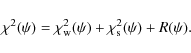
|
(18) |
The algorithm is grid-based and expresses the derivatives of the lensing potential by finite-differencing schemes. Starting from a coarse initial grid, the resolution is steadily increased until the final reconstruction is reached. At each iteration the reconstruction is regularized on the former iteration by the regularization function
The weak lensing constraints are obtained by averaging over a
certain number of background-galaxy ellipticities in every
reconstruction pixel. The error is given by the statistical scatter in
each pixel. Afterwards the reduced shear of the cluster is fitted:
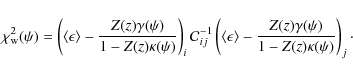
The sum over i and j runs over all reconstruction pixels, and the cosmological-weight function Z(z) describes the redshift distribution of the sources
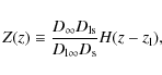
|
(20) |
where
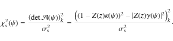
The strong lensing constraints are based on the estimated positions
of the critical curves of the galaxy cluster. They are given by the
observed arc positions and/or multiple images bracketing the critical
lines. Assuming a reconstruction pixel to be part of a critical curve,
by summing over all these pixels with index k, we find
|
(21) |
The error
A final high-resolution step is added, which is able to resolve the
positions of the critical curve estimators in greater detail. Since
there is no reliable weak lensing information on this resolution, this
step is embedded in the foregoing reconstruction by regularizing on the
former result in the cluster center:
|
(22) |
The mass analysis is then done with a convergence map, which is calculated from the reconstructed lensing potential of the cluster using Eq. (A.5).
In Fig. 8, we show the mass profiles of cluster g1-y
obtained with the weak-lensing methods described above. All the methods
perform well by providing consistent results for this particular
cluster. The mass profiles deviate from the true one by less than ![]() at all radii. The vertical lines show the position of R2500, R500, and R200,
i.e. the estimated radii enclosing over-densities of 2500, 500, and 200
times the critical density of the universe, as derived from the NFW
model that best fits the tangential shear profile. In the case of the
2D mass reconstruction method combining strong and weak lensing,
we estimated the errors on the masses by bootstrapping 24 galaxy
catalogs and by repeating the reconstruction with each of them. This is
computationally very demanding, so we reconstruct the lensing potential
a coarse grid of
at all radii. The vertical lines show the position of R2500, R500, and R200,
i.e. the estimated radii enclosing over-densities of 2500, 500, and 200
times the critical density of the universe, as derived from the NFW
model that best fits the tangential shear profile. In the case of the
2D mass reconstruction method combining strong and weak lensing,
we estimated the errors on the masses by bootstrapping 24 galaxy
catalogs and by repeating the reconstruction with each of them. This is
computationally very demanding, so we reconstruct the lensing potential
a coarse grid of
![]() pixels covering the whole cluster field (
pixels covering the whole cluster field (
![]() ).
).
![\begin{figure}
\par\includegraphics[width=7.5cm,clip]{figures/13222fig8.eps}
\end{figure}](/articles/aa/full_html/2010/06/aa13222-09/img134.png)
|
Figure 8: Results of the weak lensing analysis. Radial 2D-mass profiles of cluster g1-y, as obtained from the three different methods used in this work, namely the NFW fit to the shear profile (diamonds), the aperture mass densitometry (triangles), and the 2D mass reconstruction combining weak and strong lensing (dotted line). The solid line shows the true mass profile. The vertical lines indicate the positions of R2500, R500, and R2500 as derived from the NFW fit. The bottom panel shows the ratios between the mass profiles recovered from the lensing analysis and the true mass profile. The dotted line refers again to the SL+WL method, while the red and blue solid lines indicate the results for the NFW fit and for the aperture mass, respectively. |
| Open with DEXTER | |
3.4 X-ray
Soft band [0.7-2] keV X-ray images were created from the event files. With them we identify the regions of dense cold blobs that we mask in any further analysis. The masked regions were overlaid on the X-ray images for each cluster projection in Fig. 4. These bright point-like spots were mostly correlated to the cores of previously merged substructures. Furthermore, we excluded an inner region of 60 kpc h-1 for g51 and 70 kpc h-1 for g1 and g72 (Fig. 4) to exclude the central region affected by the overcooling problem. From the soft band image, we finally produced the surface brightness profiles using 30 annuli spanning from 23 to 400 arcsec. The surface brightness profile of the cluster g1-y is given in Fig. 9. In the same radial range, we extraced the spectra of 10-15 annuli logarithmically spaced. We subsequently analyzed the spectra in XSPEC (Arnaud 1996) using a single-temperature MEKAL model (Liedahl et al. 1995; Mewe et al. 1985) to obtain the temperature and the normalization. The values of redshift and hydrogen column density are set accordingly to the input simulation. The temperature profile of g1-y is shown in Fig. 10.
![\begin{figure}
\par\includegraphics[width=7.5cm,clip]{figures/13222fig9.eps}
\end{figure}](/articles/aa/full_html/2010/06/aa13222-09/img135.png)
|
Figure 9: Radial surface brightness profile of cluster g1-y, as derived from the analysis of the X-ray observation shown in upper middle panel of Fig. 4 (diamonds). The dotted and the dashed lines show the fits to the data obtained with the forward and with the backward methods, respectively. |
| Open with DEXTER | |
![\begin{figure}
\par\includegraphics[width=7.5cm,clip]{figures/13222fig10.eps}
\end{figure}](/articles/aa/full_html/2010/06/aa13222-09/img136.png)
|
Figure 10: Radial temperature profile of cluster g1-y, as obtained from the spectral analysis of the X-ray observation (data points). The dotted and the dashed lines show the fits to the data obtained with the forward and with the backward methods, respectively. See text for more details. |
| Open with DEXTER | |
The X-ray gas and total masses are recontructed using two different methods, here labeled backward and forward methods. In brief, starting from the observed X-ray surface brightness and the radially resolved spectroscopic temperature measurements and under the assumption of spherical geometry and hydrostatic equilibrium between the ICM and the underlying dark matter potential, the backward puts constraints on a parametric functional form of the total mass by deprojecting the observed quantities, while the forward makes direct use of the 3-D model of the gas density and temperature profiles by estimating the model parameters by projecting the profiles and fitting them to the observed ones.
We describe here the two methods in detail.
Backward method.
A functional form of the total mass has to be assumed. From this and moving backward, the profiles of the observed quantities are recovered. In this work, the NFW model in Eq. (2) is used to describe the density profile of the clusters, so that
where
|
(24) |
and
The two free parameters
![]() are constrained by minimizing
a
are constrained by minimizing
a ![]() statistic defined as
statistic defined as
where
where G is the gravitational constant,
Forward method.
By this technique, the total mass profile is recovered through directly (forward) applying the hydrostatic equilibrium equation (see Eq. (26)) once a parametric form of the gas density and temperature profiles hve been estimated. In the following analysis, we adopt the approach by Vikhlinin et al. (2006) that follows similar techniques presented in, e.g., Lewis et al. (2003) and Pratt & Arnaud (2003) and extends the number of parameters to increase the modeling freedom. In particular, the formula describing the gas density is a| |
= | (27) | |
where
![\begin{displaymath}T=T_0 \frac{(r/r_{\rm t})^{-a}}{[1+(r/r_{\rm t})^b]^{c/b}}T_{\rm Cool}.
\end{displaymath}](/articles/aa/full_html/2010/06/aa13222-09/img157.png)
|
(28) |
For these simulations, where the cool cores are well inside the excluded inner regions (see Fig. 4), we consider N2=0 and
To summarize, by using the observed X-ray surface brightness and temperature profiles,
these two methods provide: (backward method) starting from a given gas density profile,
the gas mass
![]() and the best-fit parameters
and the best-fit parameters
![]() from which a
total mass profile and a 3D temperature profiles are recovered;
(forward method) for some given parametric forms of the gas and temperature profiles, their best-fit parameters
from which
from which a
total mass profile and a 3D temperature profiles are recovered;
(forward method) for some given parametric forms of the gas and temperature profiles, their best-fit parameters
from which
![]() and
and
![]() are estimated.
In the following analysis, the results obtained from these two methods are compared
to assess the systematics in the X-ray analysis of the matter distribution.
are estimated.
In the following analysis, the results obtained from these two methods are compared
to assess the systematics in the X-ray analysis of the matter distribution.
![\begin{figure}
\par\includegraphics[width=7.5cm,clip]{figures/13222fig11.eps}
\end{figure}](/articles/aa/full_html/2010/06/aa13222-09/img161.png)
|
Figure 11: Results of the X-ray analysis. Radial 3D-mass profiles of cluster g1-y, as obtained from the forward (triangles) and from the backward methods (diamonds) used in this work. The solid line shows the true mass profile. The vertical lines indicate the positions of R2500, R500 and R2500 as derived from the lensing (see Fig. 8, dashed lines) and from the X-ray backward analyses (dotted lines). |
| Open with DEXTER | |
In Fig. 11 we show the 3D-mass profiles of cluster g1-y, obtained with both the forward and the backward methods. In the region between R2500 and R200 the two methods are consistent with each other and they underestimate the true mass profile by ![]()
![]() .
Similar results are found for the other clusters in the sample and are discussed in detail in Sect. 4.3. The vertical lines in the figure indicate the estimated sizes of R2500, R500, and R200.
Because of the mass underestimate in the X-ray case, the radii measured through
lensing are typically larger than those measured via the X-ray methods.
This is clearly shown in Fig. 12 where we report the ratio of the extimated to the true characteristic radii calculated for each cluster projection
using the weak lensing signal or the X-ray analysis.
It is worth noting that even if the X-ray method always underestimates the true
radii, this bias seem to have a quite small scatter.
On the contrary while the weak lensing is a less biased estimator, we find for it a much larger scatter.
Just for convenience in the following analysis, we compare the X-ray and the
lensing masses at the same physical radii, which we choose to be R2500,
R500, R200 as derived from lensing.
.
Similar results are found for the other clusters in the sample and are discussed in detail in Sect. 4.3. The vertical lines in the figure indicate the estimated sizes of R2500, R500, and R200.
Because of the mass underestimate in the X-ray case, the radii measured through
lensing are typically larger than those measured via the X-ray methods.
This is clearly shown in Fig. 12 where we report the ratio of the extimated to the true characteristic radii calculated for each cluster projection
using the weak lensing signal or the X-ray analysis.
It is worth noting that even if the X-ray method always underestimates the true
radii, this bias seem to have a quite small scatter.
On the contrary while the weak lensing is a less biased estimator, we find for it a much larger scatter.
Just for convenience in the following analysis, we compare the X-ray and the
lensing masses at the same physical radii, which we choose to be R2500,
R500, R200 as derived from lensing.
![\begin{figure}
\par\includegraphics[width=7.5cm,clip]{figures/13222fig12.eps}
\end{figure}](/articles/aa/full_html/2010/06/aa13222-09/img163.png)
|
Figure 12: Ratio of the estimated to the true characteristic radii calculated for each cluster projection. Squares, stars, and crosses refer to size derived using the weak lensing, the X-ray forward, and the X-ray backward method, respectively. The continuous line indicates where the true and the estimated size are equal. The top, middle, and lower panel refer to R2500, R500, and R200, respectively. |
| Open with DEXTER | |
4 Results
In this section we discuss the results of the analyses outlined in the previous sections. We start with a discussion of the 2D mass estimates obtained with the lensing techniques, and then consider the deprojection of the lensing profiles and the X-ray 3D-mass estimates. Finally, we compare lensing and X-ray mass profiles and discuss how our results match the observations.4.1 Lensing 2D mass profiles
![\begin{figure}
\par\includegraphics[width=7.5cm,clip]{figures/13222fig13.eps}
\end{figure}](/articles/aa/full_html/2010/06/aa13222-09/img164.png)
|
Figure 13:
The projected masses estimated through the strong lensing analysis vs.
the corresponding true masses of the lenses. The dotted lines
correspond to
|
| Open with DEXTER | |
![\begin{figure}
\par\includegraphics[width=7.5cm,clip]{figures/13222fig14.eps}
\end{figure}](/articles/aa/full_html/2010/06/aa13222-09/img165.png)
|
Figure 14:
The relative difference between true and estimated projected masses
as a function of the distance from the cluster centers. The results are obtained
by averaging over all the clusters in the sample. The diamonds and the triangles
refer to the simulations including and excluding the contribution of the BCG to
the lensing signal (see text for more details). The errorbars show the scatter
among all the reconstructions. The regions probed by SL are typically smaller
than |
| Open with DEXTER | |
4.1.1 Strong lensing masses
In Fig. 13, we compare the true and the estimated strong-lensing masses of all clusters in our sample. The 2D masses are measured at the limits of the strong lensing regions, given by the mean distance of the tangential images from the cluster center. The agreement between the estimated and true masses is remarkable, showing that, in most cases, strong lensing methods based on parametric modeling are accurate at the level of a few percent at predicting the projected inner mass. The worst results are obtained for clusters g51-zand g72-z, for which the offsets between the true and the estimated mass areAlthough the mass measurement is very precise at the position of the tangential
critical lines, as anticipated in Sect. 3.1, the
extrapolation of strong lensing models to larger radii such as R2500,
R500, or R200 could lead to incorrect mass estimates. In particular,
we find that the results are very sensitive to the parameterization chosen to
model the BCG, when we include the central images in the optimization. Using the
wrong model leads to biased mass estimates. In our simulations we adopted a
PIEMD, which is a broadly used profile for describing the central galaxies in
clusters. This model, however, is not adequate for describing the profile of the
BCGs in our simulations. While the PIEMD model is isothermal, i.e. the surface
density profile decreases with the distance from the center as
![]() ,
the true surface density distribution of the stars in
our numerical simulations is steeper, i.e.
,
the true surface density distribution of the stars in
our numerical simulations is steeper, i.e.
![]() .
This implies that, by fitting the lensing constraints as we do, we require that
the BCG is more spatially extended, so an additional contribution to the
central mass has to be provided by the dark matter halo. This causes us to
systematically overestimate of the halo concentration and underestimate of the
scale radius, as shown in Table 3.
For this reason, the masses extrapolated to large radii are systematically
underestimated. Such a dependence on the BCG mass has been reported recently by
() when modeling the cluster MS2137 (see
also Comerford et al. 2006).
The diamonds in Fig. 14 show the mean relative differences
between true and estimated projected masses of the clusters at different
distances from the centers. As the distance from the cluster center grows, the
amplitude of the bias in the mass estimates increases to about
.
This implies that, by fitting the lensing constraints as we do, we require that
the BCG is more spatially extended, so an additional contribution to the
central mass has to be provided by the dark matter halo. This causes us to
systematically overestimate of the halo concentration and underestimate of the
scale radius, as shown in Table 3.
For this reason, the masses extrapolated to large radii are systematically
underestimated. Such a dependence on the BCG mass has been reported recently by
() when modeling the cluster MS2137 (see
also Comerford et al. 2006).
The diamonds in Fig. 14 show the mean relative differences
between true and estimated projected masses of the clusters at different
distances from the centers. As the distance from the cluster center grows, the
amplitude of the bias in the mass estimates increases to about ![]() at a
distance of two arcmins. The size of the errorbars reflects the scatter among
the reconstructions. The scatter also grows as a function of the
distance from the center.
at a
distance of two arcmins. The size of the errorbars reflects the scatter among
the reconstructions. The scatter also grows as a function of the
distance from the center.
| Figure 15: Comparison between the weak-lensing and the true 2D-masses of all the simulated clusters. From left to right, the panels refer to the methods based on the NFW fit of the shear profile, on the aperture mass densitometry, and on the non-parametric SL+WL reconstruction of the lensing potential, respectively. Shown are the ratios between the estimated and the true masses measured at three characteristic radii, namely R2500 (diamonds), R500 (triangles), and R200 (squares), versus the cluster names. |
|
| Open with DEXTER | |
To better illustrate how the results shown above depend on the stellar
component of the lenses, we ran a new set of lensing simulations using only the
dark matter halos of the clusters as deflectors. Then, we repeated the fitting
procedure and we derived the mass profiles as done before, but without modeling
the BCGs. In this case, even extrapolating the profiles to radii much larger
than the size of the strong lensing region, we find a much smaller disagreement
between true and estimated masses. In this case, the strong
lensing masses at large radii tend to be on average only slightly higher than
the true masses (<![]() ).
).
4.1.2 Weak lensing masses
We discuss now the results obtained from the weak-lensing analysis of the clusters in our sample.
The accuracy of the mass estimates depends on the morphology of the lenses and
on their substructures.
No big substructures are contained in the cylinders in the case of cluster
g1. As shown in Fig. 1, the cluster appears regular in all
three projections. Instead, clusters g51 and g72 have more complex
morphologies; in particular, as explained above, g72 has a massive companion
(![]()
![]() Mpc) located at
Mpc) located at ![]() 2.5 h-1 Mpc from the
center. When projected along the z-axis of the simulation box, the
substructure is very close to the cluster center (
2.5 h-1 Mpc from the
center. When projected along the z-axis of the simulation box, the
substructure is very close to the cluster center (![]() 300 h-1 kpc). For
this reason, this mass clump has been included in the strong lensing model of
g72-z. Although it lies outside R200 in the projections g72-x and
g72-y, this substructure produces a significant shear that complicates the
weak lensing mass measurements of the main cluster clump, as described below.
300 h-1 kpc). For
this reason, this mass clump has been included in the strong lensing model of
g72-z. Although it lies outside R200 in the projections g72-x and
g72-y, this substructure produces a significant shear that complicates the
weak lensing mass measurements of the main cluster clump, as described below.
| Figure 16: As in Fig. 15, but comparing the estimated and true 3D-masses. |
|
| Open with DEXTER | |
Two methods assume that the lensing signal is tangential to the center of the
lens, which is assumed to coincide with the BCG. This implies that all shear is
assumed to be produced by a main cluster clump. These are the NFW fit and the
aperture mass densitometry methods. For some lenses, such as the three
projections of g1, this approximation is fairly well met. Indeed, this cluster
is free of large substructures, and the shear is dominated by the main cluster
clump. For some other lenses, such as the three projections of g72, this is
not the case. In all three projections of this cluster, the shear produced by
the secondary mass clump contributes significantly to the total shear. As a
result, the tangential shear
with respect to cluster center is smaller than it should be in the projection
along the x- and the y-axes in the absence of the secondary mass component.
When fitting the shear profile with a single NFW model or converting the shear
into a mass estimate using the aperture mass densitometry, this causes to
underestimate the mass. The amplitude of this effect grows with increasing
distance from the cluster center, because the secondary mass clump is
approached. In the case of g72-x and g72-y, using the NFW fit method, the
mass is underestimated by ![]()
![]() at R2500 and by
at R2500 and by ![]()
![]() at
R200. Similar results are found with the aperture mass densitometry. In the
case of g72-z, where the secondary clump is located near the cluster center,
the shear produced by the main cluster and by the substructure sum up. The
resulting tangential shear mimics that of a lens with a higher mass and with an
extended core, because of the offset between the two mass clump centers. As a
result, we find that the estimated M200 exceeds the true value by
at
R200. Similar results are found with the aperture mass densitometry. In the
case of g72-z, where the secondary clump is located near the cluster center,
the shear produced by the main cluster and by the substructure sum up. The
resulting tangential shear mimics that of a lens with a higher mass and with an
extended core, because of the offset between the two mass clump centers. As a
result, we find that the estimated M200 exceeds the true value by ![]()
![]() .
.
To validate our interpretation of these results, we performed the following
tests. First, we placed two NFW halos of mass
![]() and
and
![]() at a distance of
2.5 h-1 Mpc, and we calculated the shear field produced by these two mass
clumps. Then, we sampled the shear field at random galaxy positions and added
the noise due to the intrinsic galaxy ellipticities, following the method
outlined in Maturi et al. (2005). Finally we measured the tangential shear profile with
respect to the center of the most massive halo and fit it using a single NFW
profile, over a radial range similar to the one used in our numerical
simulations. We repeated the experiment after removing the least massive halo.
We find that, if the shear produced by the second halo is included in the
simulation, the masses at R2500, R500, and R200 are
underestimated with respect to the simulation including only the most massive
halo, by
at a distance of
2.5 h-1 Mpc, and we calculated the shear field produced by these two mass
clumps. Then, we sampled the shear field at random galaxy positions and added
the noise due to the intrinsic galaxy ellipticities, following the method
outlined in Maturi et al. (2005). Finally we measured the tangential shear profile with
respect to the center of the most massive halo and fit it using a single NFW
profile, over a radial range similar to the one used in our numerical
simulations. We repeated the experiment after removing the least massive halo.
We find that, if the shear produced by the second halo is included in the
simulation, the masses at R2500, R500, and R200 are
underestimated with respect to the simulation including only the most massive
halo, by ![]() ,
,
![]() ,
and
,
and ![]() ,
respectively.
This qualitatively
agrees with the results for g72-x and g72-y. In both cases, the
tangential shear profile is well-fitted by an NFW profile, i.e. with reduced
,
respectively.
This qualitatively
agrees with the results for g72-x and g72-y. In both cases, the
tangential shear profile is well-fitted by an NFW profile, i.e. with reduced
![]() .
As a second test, we placed the least massive halo at a
distance of
300 h-1 kpc from the main halo. The resulting tangential shear
profile is compared with the one produced by a single-mass component of total
mass M=M1+M2. By fitting with NFW models, we find that, in the two-halo
case, the masses at R2500, R500, and R200 are overestimated by
.
As a second test, we placed the least massive halo at a
distance of
300 h-1 kpc from the main halo. The resulting tangential shear
profile is compared with the one produced by a single-mass component of total
mass M=M1+M2. By fitting with NFW models, we find that, in the two-halo
case, the masses at R2500, R500, and R200 are overestimated by
![]() ,
,
![]() ,
and
,
and ![]() ,
respectively, with the respect to the single-halo
case. This is also in good agreement with our results for g72-z.
,
respectively, with the respect to the single-halo
case. This is also in good agreement with our results for g72-z.
For the remaining clusters, the mass estimates obtained with these two methods
are more accurate. Typically, the estimated masses deviate by ![]()
![]() from the true masses. Even in the case of g51, despite the presence of a few
substructures in the cluster surroundings, the mass estimates are in good
agreement with the input masses. The reason is that the above-mentioned
substructures are less massive than in the case of g72 and the shear is
dominated by the cluster halo.
from the true masses. Even in the case of g51, despite the presence of a few
substructures in the cluster surroundings, the mass estimates are in good
agreement with the input masses. The reason is that the above-mentioned
substructures are less massive than in the case of g72 and the shear is
dominated by the cluster halo.
The nonparametric SL+WL method does not require any assumption about the
symmetry of the lensing signal. Substructures are included in the mass model by
construction. For this reason, the SL+WL method can recover the input mass with
good precision even in the case of morphologically disturbed clusters. We find
that the deviations between estimated and true masses are typically below the
![]() level.
level.
For all the three methods, the scatter between estimated and true masses grows as a function of the radius, in agreement with Okabe et al. (2009).
4.2 Lensing 3D masses
As stated several times above, lensing measures the total mass contained in cylinders and projected on the sky. To convert the 2D-mass into 3D-mass estimates, deprojection needs to be implemented. This requires to make some assumptions on the shape of the clusters and on their 3D density profile. We assume here that clusters are spherical and that their density profile is well described by the NFW model.
Deprojection is done differently for the three methods investigated here. For the NFW fit method, we use the NFW parameters obtained from the fit of the tangential shear profile to calculate the 3D-mass profile of the lenses. For the aperture mass densitometry and for the SL+WL methods, we fit the 2D-mass profiles with projected NFW models and we use the best-fit parameters to derive the 3D-mass profiles. These 3D-profiles are shown in Fig. B.1 for the individual cluster projections.
Similar to Fig. 15, we show in Fig. 16 the
ratios between estimated and true 3D-masses at three over-density radii. It is
clear that in 3D the scatter between the estimates and the input masses is
significantly larger than in 2D. This is due to two main reasons. First, lenses
are triaxial, while we are assuming spherical symmetry during the deprojection.
The impact of triaxiality on lensing mass estimates was already highlighted by
several authors in past (e.g. Oguri et al. 2005; Gavazzi 2005). Depending on the degree of
triaxiality and on the orientation of the clusters with respect to the line of
sight, 3D-masses may result to be over- or under-estimated. In particular, we
find that, in the cases of good alignment (i.e. small angles) between the major
axis of the cluster and the projection axis, the lensing masses tend to be
systematically larger than the true masses, while the opposite occurs in those
cases where the major axis is nearly perpendicular to the line of sight. This is
shown in Fig. 17, where the lensing masses are derived with the SL+WL
method, which even in 3D seems to provide the most accurate mass estimates.
Given that the masses of ellipsoids and spheres with the same azimuthal density
profile tend to converge at large distances from their centers, the effect is
strongest for M2500 and for M500, and mildest for M200. However,
even at R200, the analysis of our sample shows that the scatter due to
triaxiality is ![]()
![]() .
Similar results are found by
Corless & King (2007).
.
Similar results are found by
Corless & King (2007).
![\begin{figure}
\par\includegraphics[width=7.5cm,clip]{figures/13222fig17.eps}
\end{figure}](/articles/aa/full_html/2010/06/aa13222-09/img184.png)
|
Figure 17: Ratio between estimated and true lensing masses as a function of the angle between the major axis of the cluster inertia ellipsoid and the axis along which the mass distribution is projected. The results are shown for the lensing masses obtained with the SL+WL method. Squares, triangles and diamonds indicate the mass measurements at R200, R500, and R2500, respectively. |
| Open with DEXTER | |
The second factor which makes the 3D lensing mass estimates so noisy is
the presence of substructures along the line of sight. Since their
distance from the lens plane is unknown, the 3D-mass estimates can be
severely affected by these mass clumps, especially if they are located
close to the cluster core in projection. The high ratio between the
estimated and the true mass of g72-z is in large part due to the presence of the massive sub-clump previously mentioned in the paper. This accounts for ![]()
![]() of the total cluster mass, but its erroneous inclusion in the central
300 h-1 kpc significantly affects the mass estimates at small radii.
of the total cluster mass, but its erroneous inclusion in the central
300 h-1 kpc significantly affects the mass estimates at small radii.
![\begin{figure}
\par\includegraphics[width=6.8cm,clip]{figures/13222fig18a.eps}\h...
...{4mm}
\includegraphics[width=6.8cm,clip]{figures/13222fig18d.eps}
\end{figure}](/articles/aa/full_html/2010/06/aa13222-09/img185.png)
|
Figure 18: Top panels: comparison between the X-ray and the true 3D-masses of all the simulated clusters. The left and the right panels refer to the forward and backward methods, respectively. Shown are the ratios between the estimated and the true masses measured at three characteristic radii, namely R2500(diamonds), R500 (triangles), and R200 (squares), as a function of the cluster name. Bottom panels: as for the upper panels, but comparing the gas masses derived from the X-ray analysis to the true gas masses of the clusters. |
| Open with DEXTER | |
Apart from this particular cluster projection, in the cases of systems without
large substructures along the line of sight, 3D-lensing masses are affected by
an intrinsic uncertainty due to triaxiality, which we estimate to be about
![]() at R200. Unfortunately, at smaller radii where the lensing
measurements of the 2D masses would be more robust, the scatter becomes larger,
since it is around
at R200. Unfortunately, at smaller radii where the lensing
measurements of the 2D masses would be more robust, the scatter becomes larger,
since it is around ![]() .
.
Recently by studying the weak lensing signal of 30
galaxy clusters observed with the SUBARU telescope, Okabe et al. (2009)
have found that the mean ratios between 3D- and 2D-masses at
![]() and
R500 are
and
R500 are
![]() and
and
![]() ,
respectively, where
,
respectively, where
![]() is the virial radius. They derive the 2D-masses using the aperture mass
densitometry method, while the 3D-masses are obtained from the NFW fits of the
shear profiles. Their sample spans a range of masses that is much wider
than covered by our sample. From their Fig. 8, we can estimate that, by limiting
the analysis to masses
is the virial radius. They derive the 2D-masses using the aperture mass
densitometry method, while the 3D-masses are obtained from the NFW fits of the
shear profiles. Their sample spans a range of masses that is much wider
than covered by our sample. From their Fig. 8, we can estimate that, by limiting
the analysis to masses
![]() and
and
![]() ,
the ratios are lower (
,
the ratios are lower (![]() 1.06 and
1.06 and ![]() 1.37 at
1.37 at
![]() and at R500, respectively).
Averaging over our sample, we find
and at R500, respectively).
Averaging over our sample, we find
![]() and
and
![]() .
These are in quite good agreement with the the ratios between the true 2D- and
3D-masses, which are
.
These are in quite good agreement with the the ratios between the true 2D- and
3D-masses, which are
![]() and
and
![]() .
From these results, we can deduce that a) on average, the ratios
between 2D- and 3D-masses are well recovered, despite triaxiality and
substructures affecting individual mass estimates, and b) the agreement
between simulations and observations is an indication that the density
profiles of real and simulated clusters are, within the errors,
compatible with each other.
.
From these results, we can deduce that a) on average, the ratios
between 2D- and 3D-masses are well recovered, despite triaxiality and
substructures affecting individual mass estimates, and b) the agreement
between simulations and observations is an indication that the density
profiles of real and simulated clusters are, within the errors,
compatible with each other.
4.3 X-ray masses
In Fig. 18 we
compare the true and estimated total (dark matter and gas) and gas only
masses for all the cluster in our sample. The left and the right panels
refer to the forward and to the backward methods described in Sect. 3.4.
The top panels show the ratios between the estimated and the true masses
measured at three characteristic radii, namely R2500 (diamonds), R500(triangles), and R200 (squares), as a function of the cluster name. A
comparison of the mass profiles at any other radius is shown in
Fig. B.1. The forward and backward methods give results which,
at the three different characteristic radii, are consistent within ![]() for
all the clusters. The reconstruction of the X-ray masses through the two
methods can differ because, while the backward method assumes a functional form
of the total density profile imposing the gas temperature profile for any given
gas density profile, the forward method reproduces the gas density and
temperature with very flexible models that, in particular in the outer regions,
can induce unstable extrapolations.
for
all the clusters. The reconstruction of the X-ray masses through the two
methods can differ because, while the backward method assumes a functional form
of the total density profile imposing the gas temperature profile for any given
gas density profile, the forward method reproduces the gas density and
temperature with very flexible models that, in particular in the outer regions,
can induce unstable extrapolations.
Table 2: Radial ranges used for fitting NFW profiles to the lensing and X-ray data, with all radii expressed in units of r200 reported in Table 1.
Table 3: The NFW concentrations and scale radii (upper and lower part of the table, respectively) resulting from the strong-lensing (Col. 4), weak-lensing (Col. 5), strong+weak lensing (Col. 6), and X-ray analyses (Cols. 7, 8 for the forward and for the backward methods) of the clusters in our sample.
For the forward method, the confidence intervals on mass profiles have been estimated by minimizing the distance between the projected models and a set of 100 random realizations of observed profiles. These profiles were obtained assuming Gaussian statistics around observed values of the surface brightness and temperature profiles with the constraint of rejecting realizations leading to non-physical solution of non-monotonically increasing mass profiles. For the backward method, errors onSimilar to what is shown in other work (see e.g. Rasia et al. 2008; Nagai et al. 2007; Rasia et al. 2006, and references therein), we find that, overall the X-ray mass estimates are biased low by 5%-20%. More quantitatively we find that, on average, both methods underestimate the true mass by 10% with a scatter of 6% almost independently of the characteristic radius considered. The most deviant mass estimate comes only from the z projection of cluster g72. This again comes from this cluster being composed by two structures that line up along the line of sight (see Fig. 1). When we fit the surface brightness profile this appears to be steeper in the center and shallower at the characteristic radius.
In the bottom panels of Fig. 18, we compare the gas
masses derived from the X-ray analysis to the true gas masses of the clusters.
Again, we find that the two methods give consistent results within ![]() errors.
Furthermore, in agreement with other work, we find that the total gas mass is
fully reconstructed (Nagai et al. 2007). More quantitatively we find
that, on average, the gas mass is recovered to better than 1% with a 3% scatter at R2500 and 7% with a 3% scatter
at R500 and R200. It is important to say that the trend to slightly
overestimate the gas mass at large radii comes from both X-ray methods
tending to slightly overestimate the cluster density profiles in the outskirts
due to the imperfect azimuthal symmetry of the cluster surface brightness at
larger radii.
The most deviant gas mass estimates is given by the z projection of cluster g72. Again this results from the same effect explained above for the mass.
errors.
Furthermore, in agreement with other work, we find that the total gas mass is
fully reconstructed (Nagai et al. 2007). More quantitatively we find
that, on average, the gas mass is recovered to better than 1% with a 3% scatter at R2500 and 7% with a 3% scatter
at R500 and R200. It is important to say that the trend to slightly
overestimate the gas mass at large radii comes from both X-ray methods
tending to slightly overestimate the cluster density profiles in the outskirts
due to the imperfect azimuthal symmetry of the cluster surface brightness at
larger radii.
The most deviant gas mass estimates is given by the z projection of cluster g72. Again this results from the same effect explained above for the mass.
4.4 NFW fit parameters
The best-fit NFW parameters for all the clusters in the sample, obtained both through the lensing and X-ray analyses in the radial ranges listed in Table 2, are summarized in Table 3. In Cols. 2 and 3, we quote the true concentrations obtained by fitting the DM-only and the total density profiles of the three clusters in the radial range between 10 h-1 kpc and r200. Below each column, we report the mean ratios of the estimated and the true parameters. These are calculated both including and neglecting the three projections of g51, which strongly bias the mean concentrations and scale radii derived from the X-ray analyses, as discussed later in the text. The numbers in parentheses are the corresponding rms values.
In Col. 4
of the table we report the best-fit concentrations and scale radii obtained for
the main cluster halo using the strong-lensing constraints. These results were
obtained by including the central images in the strong lensing modeling. As
discussed in Sect. 4.1.1, this leads to systematically overestimating
the concentration and underestimating the scale radius, being the PIEMD model
used in the SL modeling inadequate to describe the distribution of the stars in
the simulations. In particular, we note that, in some cases, the concentrations
are off by a factor of ![]() 3 with respect to the true values reported in the
second column. On average, the concentrations derived from SL alone are
almost
3 with respect to the true values reported in the
second column. On average, the concentrations derived from SL alone are
almost ![]() higher than the true concentrations of the DM-only profiles.
Conversely, the scale radii are almost
higher than the true concentrations of the DM-only profiles.
Conversely, the scale radii are almost ![]()
![]() lower. We recall that the
SL fits refer to the cluster halos, while the stars are modeled apart. Such a
bias is not present in the simulations without stars, where the average ratio
between estimated and true concentrations is around unity.
lower. We recall that the
SL fits refer to the cluster halos, while the stars are modeled apart. Such a
bias is not present in the simulations without stars, where the average ratio
between estimated and true concentrations is around unity.
The weak-lensing best-fit parameters, obtained from the fit of the shear
profiles, are given in Col. 5. The concentrations tend to be slightly higher
than those of the dark-matter distributions in the input models (
![]() )
and the scale radii are on average
)
and the scale radii are on average
![]()
![]() smaller than the input values (
smaller than the input values (
![]() ). Similar results are found by combining SL
and WL (Cols. 6). In this case the average ratio between estimated and true
concentrations is
). Similar results are found by combining SL
and WL (Cols. 6). In this case the average ratio between estimated and true
concentrations is
![]() .
For the scale radius we find
.
For the scale radius we find
![]() .
The tendency to overestimate the
concentration more when adding the SL constraints is caused by the large
contribution of the stellar and gas masses within the inner
100 h-1 kpc, as
shown in Fig. 2. We recall that in the cases of the WL and WL+SL
methods the fits are done over the total projected mass profiles, thus without
distinguishing the dark-matter component from the stellar and gas masses. To
support this interpretation, we note that the largest discrepancies with the
true concentrations arise for the cluster g51, which is characterized by an
extended strong over-cooling region in the center, where the total density
profile steepens compared to the DM only profile. This mimics a higher
concentration, because the mass profile still compatible with an NFW model.
Fitting the total density profiles of the inputs clusters indeed leads to higher
concentrations and smaller scale radii, as reported in Col. 3, which are in a
much better agreement with the results of the lensing fits.
As highlighted in the previous sections, the WL fits of some systems, like the
three projections of g72, can be strongly biased when assuming a single mass
component. Indeed, their substructures need to be properly modeled when deriving
the cluster mass from the shear signal. The SL+WL method provides a better
chance to measure the density profile, at least in some cases, like g72-x and
g72-y, where the large substructure lying at the edge of the cluster virial
region is by construction properly modeled. For g72-z, where the substructure
is near the cluster core, a correct fit of the projected mass distribution
would also require multiple mass components for the SL+WL method.
.
The tendency to overestimate the
concentration more when adding the SL constraints is caused by the large
contribution of the stellar and gas masses within the inner
100 h-1 kpc, as
shown in Fig. 2. We recall that in the cases of the WL and WL+SL
methods the fits are done over the total projected mass profiles, thus without
distinguishing the dark-matter component from the stellar and gas masses. To
support this interpretation, we note that the largest discrepancies with the
true concentrations arise for the cluster g51, which is characterized by an
extended strong over-cooling region in the center, where the total density
profile steepens compared to the DM only profile. This mimics a higher
concentration, because the mass profile still compatible with an NFW model.
Fitting the total density profiles of the inputs clusters indeed leads to higher
concentrations and smaller scale radii, as reported in Col. 3, which are in a
much better agreement with the results of the lensing fits.
As highlighted in the previous sections, the WL fits of some systems, like the
three projections of g72, can be strongly biased when assuming a single mass
component. Indeed, their substructures need to be properly modeled when deriving
the cluster mass from the shear signal. The SL+WL method provides a better
chance to measure the density profile, at least in some cases, like g72-x and
g72-y, where the large substructure lying at the edge of the cluster virial
region is by construction properly modeled. For g72-z, where the substructure
is near the cluster core, a correct fit of the projected mass distribution
would also require multiple mass components for the SL+WL method.
Comparable estimates of c and ![]() are obtained with the two X-ray
techniques. Even the X-ray analysis probes the total mass distribution,
including the gas and the stars. We note that, using the backward method,
the concentration and the scale radius are obtained
as best-fit parameters that minimize the reconstructed temperature profile with respect to the
observed values, whereas using the forward method let us estimate them
with a-posteriori
fit with a NFW functional form performed in the radial range
0.7-1.4 h-1 Mpc on the mass model obtained
by applying the hydrostatic equilibrium equation to the gas density and
temperature models described in Eqs. (27) and (28), respectively.
Overall, the deviations from the true estimates go in the same direction: in g1, c is underestimated
consistently by a factor 0.7-0.8, with a corresponding overestimate of
are obtained with the two X-ray
techniques. Even the X-ray analysis probes the total mass distribution,
including the gas and the stars. We note that, using the backward method,
the concentration and the scale radius are obtained
as best-fit parameters that minimize the reconstructed temperature profile with respect to the
observed values, whereas using the forward method let us estimate them
with a-posteriori
fit with a NFW functional form performed in the radial range
0.7-1.4 h-1 Mpc on the mass model obtained
by applying the hydrostatic equilibrium equation to the gas density and
temperature models described in Eqs. (27) and (28), respectively.
Overall, the deviations from the true estimates go in the same direction: in g1, c is underestimated
consistently by a factor 0.7-0.8, with a corresponding overestimate of ![]() up to a factor 1.45, if compared with the true concentrations obtained by
fitting the input total mass distributions of the clusters.
The same considerations apply to g72, apart from g72-z, where the
concentration (scale radius)
is estimated higher (lower) than
up to a factor 1.45, if compared with the true concentrations obtained by
fitting the input total mass distributions of the clusters.
The same considerations apply to g72, apart from g72-z, where the
concentration (scale radius)
is estimated higher (lower) than
![]() (
(
![]() )
by about 15 per cent as a consequence of the alignment
along the line of sight of the two main clumps. More critical is the case of
g51, where both the X-ray
methods provide a measure of the concentration that is twice
)
by about 15 per cent as a consequence of the alignment
along the line of sight of the two main clumps. More critical is the case of
g51, where both the X-ray
methods provide a measure of the concentration that is twice
![]() ,
again because of the large contribution
of the cool substructures in the central regions, as also shown from the overestimate of the total mass obtained
through X-ray analysis within R2500 (see Fig. 18). Although we attempted to
mask it in the X-ray analysis, the over-cooling region in this cluster is very
extended, thus it is still affecting the mass reconstruction (see
Fig. B.1 in Appendix B). On average the
X-ray concentrations are
,
again because of the large contribution
of the cool substructures in the central regions, as also shown from the overestimate of the total mass obtained
through X-ray analysis within R2500 (see Fig. 18). Although we attempted to
mask it in the X-ray analysis, the over-cooling region in this cluster is very
extended, thus it is still affecting the mass reconstruction (see
Fig. B.1 in Appendix B). On average the
X-ray concentrations are ![]()
![]() and
and ![]()
![]() lower than
lower than
![]() and
and
![]() ,
respectively, if the three
projections of g51 are not included.
,
respectively, if the three
projections of g51 are not included.
4.5 Lensing vs. X-ray 3D mass profiles
Finally, we attempted a comparison between the lensing and the X-ray mass
estimates. First of all, given the results discussed above, it is not surprising
that lensing and X-ray mass estimates in individual galaxy clusters can differ
by up to ![]() .
This is clear in Fig. 19,
where the lensing masses
are shown as a function of their X-ray equivalents. The lensing masses
were
obtained with the SL+WL method. The X-ray masses were obtained with the
forward
method. The discrepancies in the simulated sample are consistent with
those
observed in several galaxy clusters. As an example, we overplot with
asterisks the mass measurements of a sample of 18 galaxy clusters
reported by
Mahdavi et al. (2008) (M08 in the following discussion).
.
This is clear in Fig. 19,
where the lensing masses
are shown as a function of their X-ray equivalents. The lensing masses
were
obtained with the SL+WL method. The X-ray masses were obtained with the
forward
method. The discrepancies in the simulated sample are consistent with
those
observed in several galaxy clusters. As an example, we overplot with
asterisks the mass measurements of a sample of 18 galaxy clusters
reported by
Mahdavi et al. (2008) (M08 in the following discussion).
Several recent studies seem to agree on the fact that the lensing masses are on
average higher than the X-ray masses. For example, analyzing a sample of 19clusters observed with SUBARU and XMM-Newton, Zhang et al. (2008)
find that
![]() .
M08 report similar
results. In particular, they find a trend in the ratio between lensing and X-ray
masses as a function of the overdensity radius. While X-ray and the lensing
masses are consistent with each other at R2500 (
.
M08 report similar
results. In particular, they find a trend in the ratio between lensing and X-ray
masses as a function of the overdensity radius. While X-ray and the lensing
masses are consistent with each other at R2500 (
![]() ), their mean ratio becomes
), their mean ratio becomes
![]() at
R500. Correcting for excess correlated structure outside the virial radius,
they find
at
R500. Correcting for excess correlated structure outside the virial radius,
they find
![]() and
and
![]() .
Very recently when studying a sample of
12 clusters divided into relaxed and unrelaxed on the basis of their X-ray
morphology, Zhang et al. (2010) (Z09 in the
following) have also found that the weak
lensing masses exceed the X-ray masses at large radii (or low overdensities),
while they are comparable at small radii (or high overdensities). However, they
measure a shallower but still significant radial evolution of
.
Very recently when studying a sample of
12 clusters divided into relaxed and unrelaxed on the basis of their X-ray
morphology, Zhang et al. (2010) (Z09 in the
following) have also found that the weak
lensing masses exceed the X-ray masses at large radii (or low overdensities),
while they are comparable at small radii (or high overdensities). However, they
measure a shallower but still significant radial evolution of
![]() compared to M08. For the subsample of relaxed clusters, they find
compared to M08. For the subsample of relaxed clusters, they find
![]() and
and
![]() on average, while for the whole sample of
objects they find
on average, while for the whole sample of
objects they find
![]() and
and
![]() .
This trend is interpreted as an
indication of the lack of hydrostatic equilibrium in galaxy clusters
(Churazov et al. 2008).
.
This trend is interpreted as an
indication of the lack of hydrostatic equilibrium in galaxy clusters
(Churazov et al. 2008).
We repeat here the analysis of M08 and Z09 using our simulated clusters. Following the terminology of M08, we indicate with ![]() the ratio between the X-ray and 3D-lensing masses for a particular overdensity
the ratio between the X-ray and 3D-lensing masses for a particular overdensity ![]() .
We measure
.
We measure
![]() for
for
![]() ,
1000, 500, and 200. Consistently with M08 and Z09, we estimate
,
1000, 500, and 200. Consistently with M08 and Z09, we estimate
![]() by minimizing a
by minimizing a ![]() statistic defined as
statistic defined as
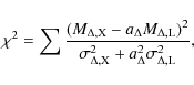
|
(29) |
where
![\begin{figure}
\par\includegraphics[width=7.5cm,clip]{figures/13222fig19.eps}
\end{figure}](/articles/aa/full_html/2010/06/aa13222-09/img307.png)
|
Figure 19:
Lensing vs. X-ray masses within R2500 (diamonds), R500 (triangles), and R200
(squares). The asterisks show the mass estimates published by M08 for a
sample of 18 galaxy clusters. The dashed lines correspond to
|
| Open with DEXTER | |
The important question that arises now is whether the ratio between lensing and
X-ray masses is a robust indicator of the lack of hydrostatic equilibrium in the
simulated clusters. This can be checked easily by measuring the mass profile of
the simulated clusters using the hydrostatic equilibrium approximation. For
doing this, we plugged the gas density and the temperature profiles measured
from the particle distributions into the hydrostatic equilibrium equation and
derived the mass
![]() .
This mass should be recovered by the X-ray
analysis; i.e.,
.
This mass should be recovered by the X-ray
analysis; i.e., ![]() is a measurement of
is a measurement of
![]() .
This mass is
compared to the true mass
.
This mass is
compared to the true mass
![]() as in Rasia et al. (2004). By considering the
three clusters, we obtained the median profile of the ratio between hydrostatic
equilibrium and total mass, shown in Fig. 20.
For comparison, we indicate the ratios between X-ray and true
masses at each overdensity radius.
In these simulations, the median
as in Rasia et al. (2004). By considering the
three clusters, we obtained the median profile of the ratio between hydrostatic
equilibrium and total mass, shown in Fig. 20.
For comparison, we indicate the ratios between X-ray and true
masses at each overdensity radius.
In these simulations, the median
![]() is
is ![]() 0.9between R2500 and R1000, and then it decreases to 0.84 and 0.8 at
R500 and R200. The X-ray masses are compatible (within the
0.9between R2500 and R1000, and then it decreases to 0.84 and 0.8 at
R500 and R200. The X-ray masses are compatible (within the ![]() confidence limit) with
confidence limit) with
![]() .
The mass derived with the backward method
declines more steeply than what was obtained with the forward method as
.
The mass derived with the backward method
declines more steeply than what was obtained with the forward method as
![]() decreases, and seems to follow the behavior of
decreases, and seems to follow the behavior of
![]() more closely, although the differences are not significant given the
error-bars.
more closely, although the differences are not significant given the
error-bars.
![]() is also compatible with
is also compatible with
![]() .
This is true only at the
.
This is true only at the ![]() significance level for
significance level for
![]() .
Thus, we conclude that lensing and X-ray observations and their comparison
to the simulations can provide important information on the physics of the gas
in galaxy clusters. Although we have considered a small sample of
clusters, averaging over several objects significantly reduces the impact of
triaxiality. Indeed, at all overdiensities,
.
Thus, we conclude that lensing and X-ray observations and their comparison
to the simulations can provide important information on the physics of the gas
in galaxy clusters. Although we have considered a small sample of
clusters, averaging over several objects significantly reduces the impact of
triaxiality. Indeed, at all overdiensities,
![]() is very
similar to
is very
similar to
![]() ,
indicating that
,
indicating that
![]() on average.
on average.
In Table 4 we
report the mean, the rms, the median,
the first and the third quartiles, and the minimal and maximal values
of the distributions of several mass ratios obtained via lensing and
X-ray analyses and from the input simulations. The lensing masses are
measured with the SL+WL method. For the X-ray masses we use both the
forward and the backward methods. Not only do we compare 3D vs.
3D masses, but we also compare 3D vs. 2D mass estimates and
vice-versa. We note that triaxiality and substructure affect the
2D X-ray mass estimates consistently to the 3D lensing mass
estimates. For example the rms of the ratio
![]() is
is ![]()
![]() ,
similar to the rms of the ratio
,
similar to the rms of the ratio
![]() .
Not surprisingly, the mass ratio that
has the smaller scatter is
.
Not surprisingly, the mass ratio that
has the smaller scatter is
![]() ,
whose
rms is
,
whose
rms is ![]()
![]() .
However, the radial dependence of this mass
ratio is stronger than for
.
However, the radial dependence of this mass
ratio is stronger than for
![]() or
or
![]() as indicated by the variation of the mean and of
the median as a function of the overdensity
as indicated by the variation of the mean and of
the median as a function of the overdensity ![]() .
Obviously, the
mass ratio affected by the largest scatter is
.
Obviously, the
mass ratio affected by the largest scatter is
![]() (
(![]()
![]() ).
).
Table 4: Summary of the comparison between lensing, X-ray, and true masses.
5 Summary and conclusions
![\begin{figure}
\par\includegraphics[width=7.5cm,clip]{figures/13222fig20.eps}
\end{figure}](/articles/aa/full_html/2010/06/aa13222-09/img336.png)
|
Figure 20:
Ratio between X-ray and lensing masses as a function of the
overdensity |
| Open with DEXTER | |
In this paper, we have tested several methods of deriving the mass of galaxy clusters via lensing and X-ray observations. To do so, we used two pipelines for simulating observations of galaxy clusters obtained from N-body and hydrodynamical simulations. These are the code SkyLens, which produces mock observations with a variety of telescopes in the optical bands, including lensing effects by matter along the line of sight, and the code XMAS, which allows mimicking of X-ray observations of galaxy clusters with the Chandra and the XMM-Newton telescopes. In our analysis, we used three massive galaxy clusters at redshifts between z=0.2335 and z=0.297. Each cluster was projected along three orthogonal axes and each projection was analyzed individually. For each cluster projection, we carried out both the lensing and the X-ray analysis using standard techniques to derive the mass profiles.
Our results can be summarized as follows.
- Strong lensing parametric mass reconstructions provide very accurate
estimates of the projected mass, but only in the regions probed by the strong
lensing features. Our simulations show that, within the Einstein rings, the
input masses are recovered with an accuracy of

 .
For most cases,
the measured masses differ from the input ones by only a few percent. The
precision depends on the complexity of the lens and on the number of lensing
constraints available. For example, using central images improves the mass
estimates in the very inner regions. On the other hand, extrapolating the mass
models to radii larger than those probed by strong lensing may easily result in
mass estimates that are wrong by up to
.
For most cases,
the measured masses differ from the input ones by only a few percent. The
precision depends on the complexity of the lens and on the number of lensing
constraints available. For example, using central images improves the mass
estimates in the very inner regions. On the other hand, extrapolating the mass
models to radii larger than those probed by strong lensing may easily result in
mass estimates that are wrong by up to  .
In particular, the assumptions
made for modeling the star distribution in the BCG affect the mass profiles at
large radii.
Although the very central regions of numerically simulated clusters may be not
representative of those of real clusters, given the uncertainties on the
treatment of small-scale physics of the intracluster gas, our results warn
against potential biases that may affect the strong lensing mass estimates.
.
In particular, the assumptions
made for modeling the star distribution in the BCG affect the mass profiles at
large radii.
Although the very central regions of numerically simulated clusters may be not
representative of those of real clusters, given the uncertainties on the
treatment of small-scale physics of the intracluster gas, our results warn
against potential biases that may affect the strong lensing mass estimates.
- Weak lensing methods for measuring the projected mass perform well with
galaxy clusters characterized by regular mass distributions, i.e. without
massive substructures that produce a significant shear. If present, such
substructures need to be properly modeled. If not, the cluster masses can be
over- or under-estimated by up to
 ,
when assuming that the shear signal is
tangential to a unique mass center. Nonparametric methods combining weak and
strong lensing, which by construction do not assume any symmetry in the lensing
signal, perform well even in the case of clusters disturbed by massive
substructures. The mass estimates at R2500, R500, and R200 are
typically recovered within a
accuracy, being more accurate at the
smallest radii.
,
when assuming that the shear signal is
tangential to a unique mass center. Nonparametric methods combining weak and
strong lensing, which by construction do not assume any symmetry in the lensing
signal, perform well even in the case of clusters disturbed by massive
substructures. The mass estimates at R2500, R500, and R200 are
typically recovered within a
accuracy, being more accurate at the
smallest radii.
- Deprojection of the lensing masses introduces a significant scatter in the ratio between estimated and true masses. Cluster triaxiality causes that the accuracy of 3D-mass estimates depends on the orientation of the lens with respect to the line of sight. For clusters whose major axis points towards the observer the 3D-mass is over-estimated, while the opposite happens for clusters oriented perpedicularly to the line of sight. Cluster substructures also cause errors during the deprojection, as the distance of the substructures from the cluster center along the line of sight is unknown.
- X-ray masses are typically biased low by
 due to the lack of
hydrostatic equilibrium in the simulated clusters. The average bias between
R2500 and R200 is
due to the lack of
hydrostatic equilibrium in the simulated clusters. The average bias between
R2500 and R200 is 
 .
In fact, the accretion of material from
the surroundings during the cluster formation process causes bulk motions that
contribute to the pressure support of the gas. As shown in previous works, this
effect is radial dependent, i.e. it is stronger in the outer regions. We
investigated whether the ratio of X-ray-to-lensing masses
.
In fact, the accretion of material from
the surroundings during the cluster formation process causes bulk motions that
contribute to the pressure support of the gas. As shown in previous works, this
effect is radial dependent, i.e. it is stronger in the outer regions. We
investigated whether the ratio of X-ray-to-lensing masses
 can be
used as a tracer of hydrostatic equilibrium. By averaging over the sample, we
find that this ratio indeed reproduces the lack of hydrostatic equilibrium
in the input simulations, although the number of available clusters is
limited and despite the effects of triaxiality and substructures which affect
the cluster 3D-mass estimates.
can be
used as a tracer of hydrostatic equilibrium. By averaging over the sample, we
find that this ratio indeed reproduces the lack of hydrostatic equilibrium
in the input simulations, although the number of available clusters is
limited and despite the effects of triaxiality and substructures which affect
the cluster 3D-mass estimates.
- The gas mass is reconstructed well within the region from which we can
extract a surface brightness profile.
Almost indipendently of the dynamical state of the cluster, the gas mass can be
recovered, on average, with an average deviation of
 at R2500 and
 between R500 and R200.
These results indicate that the comparison between lensing and X-ray mass
estimates in individual systems can be very misleading, because these two
observables probe different quantities. While lensing probes the matter
projected along the line of sight to the clusters, the X-ray emission from the
intracluster gas probes the 3D gravitational potential. Thus, a
direct comparison between lensing and X-ray masses is possible only in those
systems which are characterized by high degrees of spherical symmetry.
Additional complications are caused by substructures, which largely affect the
weak lensing measurements, at least using some methods of converting the shear
into a mass estimate. Combining strong and weak lensing, we obtained on average
a very small bias in the mass estimates (![]()
![]() ), but the scatter is fairly
high (
), but the scatter is fairly
high (![]()
![]() ). In contrast, X-ray masses are affected by a more
substantial bias (
). In contrast, X-ray masses are affected by a more
substantial bias (![]()
![]() ), but the scatter is smaller by almost a factor of
three.
), but the scatter is smaller by almost a factor of
three.
Finally, strong lensing alone provides mass estimates that are reliable only in a very small region around the cluster core, which cannot be probed by X-ray. Extrapolating the strong lensing mass models to the radii probed by X-ray (and vice-versa) may result in significant mismatches between mass estimates. Note, however, that the difficulty of fitting the strong lensing data in simulations with cooling and star formation with the approximations that are commonly used in observations is very likely caused by the unrealistic core structure of the simulated clusters.
Nevertheless, it is remarkable that,
by averaging over the whole sample, we have been able to reproduce the
ratio between true and hydrostatic equilibrium masses seen in the
simulations, under the assumption that the former is given by lensing
and the latter by X-ray. This suggests that, with a sufficiently large
sample of clusters with wide-field imaging and X-ray observations, the
impact of several noises affecting the mass estimates can be
reduced. This is positive news that suggests that weak lensing masses
may be used as reliable calibrators for the scaling relations
involving the X-ray observables, such as the
![]() ,
the
,
the
![]() ,
and
the
,
and
the
![]() relations. Moreover, the scatter due to triaxiality in the
calibration can potentially be reduced.
In fact, although its radial dependence is stronger, the ratio between
3D X-ray masses and 2D lensing masses is affected by a smaller
scatter than the ratio between 3D or 2D X-ray and lensing masses.
relations. Moreover, the scatter due to triaxiality in the
calibration can potentially be reduced.
In fact, although its radial dependence is stronger, the ratio between
3D X-ray masses and 2D lensing masses is affected by a smaller
scatter than the ratio between 3D or 2D X-ray and lensing masses.
We acknowledge financial contribution from contracts ASI-INAF I/023/05/0, ASI-INAF I/088/06/0, and INFN PD51. Support for this work was also provided by NASA through Chandra Postdoctoral Fellowship grant number PF5-70042 awarded by the Chandra X-ray Center, which is operated by the Smithsonian Astrophysical Observatory for NASA under the contract NAS8-03060. E.R. acknoweldges the Michigan Society of Fellows. We are grateful to L. Moscardini for having carefully read the manuscript and provided useful comments. M.M. thanks Yu-Ying Zhang and collaborators for providing a draft of their paper. M.M. thanks the Institut für Theoretische Astrophysik of the University of Heidelberg for hospitality during the preparation of this manuscript. The work was performed under the HPC-EUROPA2 project (project number: 228398) with the support of the European Commission - Capacities Area - Research Infrastructures. We are grateful to Y. Suto and S. Miyazaki for their help implementing the Subaru interface in the SkyLens simulator. M.M. thanks Paolo for his cooperation during the preparation of the manuscript.
Appendix A: Lensing definitions
In this section, we summarize some lensing definitions that will be useful in the rest of the paper.
We start with an isolated
lens whose surface-mass density is
![]() at the angular
position
at the angular
position
![]() on the sky. Its lensing potential is
on the sky. Its lensing potential is
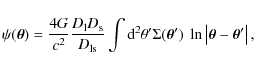
|
(A.1) |
where
The image positions
For sources much smaller than the typical scales on which the lens properties vary, the lens mapping can be linearized. The deformation of images with respect to the source is then given by the Jacobian matrix
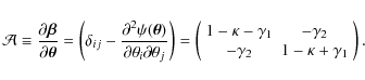
Here,
i.e. the surface-mass density scaled by its critical value
The distortion is described by the two components of the shear,
which are combined into the complex shear

|
(A.8) |
The inverse of the Jacobian determinant defines the magnification factor
|
(A.9) |
The loci on the image plane where
| (A.10) | ||
| (A.11) |
The inverses of the eigenvalues of the Jacobian matrix define the tangential and the radial magnifications: images forming close to the tangential or to the radial critical lines are highly elongated tangentially or perpendicularly to the critical lines, respectively. The critical lines are mapped onto the caustics on the source plane, via the lens equation. The caustics encompass regions of the source plane, which are characterized by different multiplicities of the images.
Outside critical curves, image ellipticities are determined by the
complex reduced shear
In the weak-lensing limit,
Source and image shapes are quantified by the complex ellipticity

|
(A.13) |
where a and b are the semi-major and semi-minor axes of an ellipse fitting the object's surface-brightness distribution. The position angle of the ellipse's major axis is
A sufficiently small source with ellipticity
![]() is
imaged to have an ellipticity
is
imaged to have an ellipticity

where the asterisk denotes complex conjugation. This equation illustrates that the lensing distortion is determined by the reduced shear, which is the only lensing quantity directly accessible through measurements of galaxy ellipticities alone.
Appendix B: Individual mass profiles
In this section we show the 3D-mass profiles (normalized to the true mass
profiles) of each individual cluster projection in our sample. This allows the
reader to compare the mass estimates at any radius different from R2500,
R500, and R200, which are already discussed in the paper. The profiles
are displayed in Fig. B.1 for all the lensing and the X-ray
methods. Additionally, we also show the mass profiles derived from the true gas
and temperature profiles under the assumption of hydrostatic equilibrium. These
last curves are quite noisy, especially in the case of g72, because we did
not apply any smoothing to the data. In the case of g51, the extended cooling
region in the cluster center causes the hydrostatic mass
![]() to be
higher than the true mass. The X-ray derived profiles reproduce the trends
seen in the
to be
higher than the true mass. The X-ray derived profiles reproduce the trends
seen in the
![]() profiles although some differences are present. While
we mask many cold blobs in the simulated observations, we are not
removing these structures from the input clusters when calculating
profiles although some differences are present. While
we mask many cold blobs in the simulated observations, we are not
removing these structures from the input clusters when calculating
![]() .
Thus, some differences between the profiles are expected.
.
Thus, some differences between the profiles are expected.
![\begin{figure}
\par\includegraphics[width=5cm,clip]{figures/13222fig21a.eps}\hsp...
...e*{4mm}
\includegraphics[width=5cm,clip]{figures/13222fig21i.eps}
\end{figure}](/articles/aa/full_html/2010/06/aa13222-09/img372.png)
|
Figure B.1: Ratios between the mass profiles recovered from the lensing and the X-ray analyses and the true 3D mass profiles of each cluster. The meaning of each line is explained in the legend. The vertical dashed lines in each panel mark the positions of R2500, R500, and R200, as derived from the lensing analysis (see text for more details). |
| Open with DEXTER | |
References
- Allen, S. 1998, MNRAS, 296, 392 [NASA ADS] [CrossRef] [Google Scholar]
- Allen, S. W., Ettori, S., & Fabian, A. C. 2001, MNRAS, 324, 877 [NASA ADS] [CrossRef] [Google Scholar]
- Allen, S. W., Rapetti, D. A., Schmidt, R. W., et al. 2008, MNRAS, 383, 879 [NASA ADS] [CrossRef] [Google Scholar]
- Allen, S. W., Schmidt, R. W., Ebeling, H., Fabian, A. C., & van Speybroeck, L. 2004, MNRAS, 353, 457 [NASA ADS] [CrossRef] [Google Scholar]
- Ameglio, S., Borgani, S., Pierpaoli, E., et al. 2009, MNRAS, 394, 479 [NASA ADS] [CrossRef] [Google Scholar]
- Arnaud, K. A. 1996, in Astronomical Data Analysis Software and Systems V, ed. G. H. Jacoby, & J. Barnes, ASP Conf. Ser., 101, 17 [Google Scholar]
- Aubert, D., Amara, A., & Metcalf, R. B. 2007, MNRAS, 376, 113 [NASA ADS] [CrossRef] [Google Scholar]
- Bartelmann, M. 1995, A&A, 299, 11 [NASA ADS] [Google Scholar]
- Bartelmann, M. 1996, A&A, 313, 697 [NASA ADS] [Google Scholar]
- Bartelmann, M., & Schneider, P. 2001, Phys. Rep., 340, 291 [NASA ADS] [CrossRef] [Google Scholar]
- Bartelmann, M., & Steinmetz, M. 1996, MNRAS, 283, 431 [NASA ADS] [Google Scholar]
- Beckwith, S. V. W., Stiavelli, M., Koekemoer, A. M., et al. 2006, AJ, 132, 1729 [NASA ADS] [CrossRef] [Google Scholar]
- Benítez, N. 2000, ApJ, 536, 571 [NASA ADS] [CrossRef] [Google Scholar]
- Bradac, M., Erben, T., Schneider, P., et al. 2005, A&A, 437, 49 [NASA ADS] [CrossRef] [EDP Sciences] [Google Scholar]
- Buote, D. A., Gastaldello, F., Humphrey, P. J., et al. 2007, ApJ, 664, 123 [NASA ADS] [CrossRef] [Google Scholar]
- Cen, R. 1997, ApJ, 485, 39 [NASA ADS] [CrossRef] [Google Scholar]
- Churazov, E., Forman, W., Vikhlinin, A., et al. 2008, MNRAS, 388, 1062 [NASA ADS] [CrossRef] [Google Scholar]
- Clowe, D., Gonzalez, A., & Markevitch, M. 2004, ApJ, 604, 596 [NASA ADS] [CrossRef] [Google Scholar]
- Clowe, D., Luppino, G. A., Kaiser, N., Henry, J. P., & Gioia, I. M. 1998, ApJ, 497, L61 [NASA ADS] [CrossRef] [Google Scholar]
- Coe, D., Benítez, N., Sánchez, S. F., et al. 2006, AJ, 132, 926 [NASA ADS] [CrossRef] [Google Scholar]
- Comerford, J. M., Meneghetti, M., Bartelmann, M., & Schirmer, M. 2006, ApJ, 642, 39 [NASA ADS] [CrossRef] [Google Scholar]
- Comerford, J. M., & Natarajan, P. 2007, MNRAS, 379, 190 [NASA ADS] [CrossRef] [Google Scholar]
- Corless, V. L., & King, L. J. 2007, MNRAS, 380, 149 [NASA ADS] [CrossRef] [Google Scholar]
- Dolag, K., Vazza, F., Brunetti, G., & Tormen, G. 2005, MNRAS, 364, 753 [NASA ADS] [CrossRef] [Google Scholar]
- Donnarumma, A., Ettori, S., Meneghetti, M., & Moscardini, L. 2009, MNRAS, 398, 438 [NASA ADS] [CrossRef] [Google Scholar]
- Eisenstein, D. J., Zehavi, I., Hogg, D. W., et al. 2005, ApJ, 633, 560 [NASA ADS] [CrossRef] [Google Scholar]
- Ettori, S., & Lombardi, M. 2003, A&A, 398, L5 [NASA ADS] [CrossRef] [EDP Sciences] [Google Scholar]
- Ettori, S., De Grandi, S., & Molendi, S. 2002, A&A, 391, 841 [NASA ADS] [CrossRef] [EDP Sciences] [Google Scholar]
- Ettori, S., Tozzi, P., & Rosati, P. 2003, A&A, 398, 879 [NASA ADS] [CrossRef] [EDP Sciences] [Google Scholar]
- Evrard, A. E., Metzler, C. A., & Navarro, J. F. 1996, ApJ, 469, 494 [NASA ADS] [CrossRef] [Google Scholar]
- Fahlman, G., Kaiser, N., Squires, G., & Woods, D. 1994, ApJ, 437, 56 [NASA ADS] [CrossRef] [Google Scholar]
- Gardini, A., Rasia, E., Mazzotta, P., et al. 2004, MNRAS, 351, 505 [NASA ADS] [CrossRef] [Google Scholar]
- Gavazzi, R. 2005, A&A, 443, 793 [NASA ADS] [CrossRef] [EDP Sciences] [Google Scholar]
- Giavalisco, M., Ferguson, H. C., Koekemoer, A. M., et al. 2004, ApJ, 600, L93 [NASA ADS] [CrossRef] [Google Scholar]
- Golse, G., Kneib, J.-P., & Soucail, G. 2002, A&A, 387, 788 [NASA ADS] [CrossRef] [EDP Sciences] [Google Scholar]
- Henriksen, M. J., & Mushotzky, R. F. 1986, ApJ, 302, 287 [NASA ADS] [CrossRef] [Google Scholar]
- Hoekstra, H. 2001, A&A, 370, 743 [NASA ADS] [CrossRef] [EDP Sciences] [Google Scholar]
- Hoekstra, H. 2003, MNRAS, 339, 1155 [NASA ADS] [CrossRef] [Google Scholar]
- Hoekstra, H. 2007, MNRAS, 379, 317 [NASA ADS] [CrossRef] [Google Scholar]
- Hoekstra, H., Franx, M., Kuijken, K., & Squires, G. 1998, ApJ, 504, 636 [NASA ADS] [CrossRef] [Google Scholar]
- Jenkins, A., Frenk, C., White, S., et al. 2001, MNRAS, 321, 372 [NASA ADS] [CrossRef] [MathSciNet] [Google Scholar]
- Jullo, E., Kneib, J.-P., Limousin, M., et al. 2007, New J. Phys., 9, 447 [Google Scholar]
- Kaiser, N., Squires, G., & Broadhurst, T. 1995, ApJ, 449, 460 [NASA ADS] [CrossRef] [Google Scholar]
- Kneib, J., Mellier, Y., Fort, B., & Mathez, G. 1993, A&A, 273, 367 [NASA ADS] [Google Scholar]
- Komatsu, E., Dunkley, J., Nolta, M. R., et al. 2009, ApJS, 180, 330 [NASA ADS] [CrossRef] [Google Scholar]
- Kravtsov, A. V., Vikhlinin, A., & Nagai, D. 2006, ApJ, 650, 128 [NASA ADS] [CrossRef] [Google Scholar]
- Lau, E. T., Kravtsov, A. V., & Nagai, D. 2009, ApJ, 705, 1129 [NASA ADS] [CrossRef] [Google Scholar]
- Liedahl, D. A., Osterheld, A. L., & Goldstein, W. H. 1995, ApJ, 438, L115 [NASA ADS] [CrossRef] [Google Scholar]
- Limousin, M., Richard, J., Jullo, E., et al. 2007, ApJ, 668, 643 [NASA ADS] [CrossRef] [Google Scholar]
- Luppino, G. A., & Kaiser, N. 1997, ApJ, 475, 20 [NASA ADS] [CrossRef] [Google Scholar]
- Mahdavi, A., Hoekstra, H., Babul, A., & Henry, J. P. 2008, MNRAS, 384, 1567 [NASA ADS] [CrossRef] [Google Scholar]
- Mantz, A., Allen, S. W., & Rapetti, D. 2009a, MNRAS, accepted [arXiv:0911.1788] [Google Scholar]
- Mantz, A., Allen, S. W., Rapetti, D., & Ebeling, H. 2009b, MNRAS, submitted [arXiv:0909.3098] [Google Scholar]
- Markevitch, M., Gonzalez, A. H., Clowe, D., et al. 2004, ApJ, 606, 819 [NASA ADS] [CrossRef] [Google Scholar]
- Maturi, M., Meneghetti, M., Bartelmann, M., Dolag, K., & Moscardini, L. 2005, A&A, 442, 851 [NASA ADS] [CrossRef] [EDP Sciences] [Google Scholar]
- Medezinski, E., Broadhurst, T., Umetsu, K., et al. 2007, ApJ, 663, 717 [NASA ADS] [CrossRef] [Google Scholar]
- Meneghetti, M., Argazzi, R., Pace, F., et al. 2007, A&A, 461, 25 [NASA ADS] [CrossRef] [EDP Sciences] [Google Scholar]
- Meneghetti, M., Bartelmann, M., & Moscardini, L. 2003a, MNRAS, 346, 67 [NASA ADS] [CrossRef] [Google Scholar]
- Meneghetti, M., Bartelmann, M., & Moscardini, L. 2003b, MNRAS, 340, 105 [NASA ADS] [CrossRef] [Google Scholar]
- Meneghetti, M., Melchior, P., Grazian, A., et al. 2008, A&A, 482, 403 [NASA ADS] [CrossRef] [EDP Sciences] [Google Scholar]
- Merten, J., Cacciato, M., Meneghetti, M., Mignone, C., & Bartelmann, M. 2009, A&A, 500, 681 [NASA ADS] [CrossRef] [EDP Sciences] [Google Scholar]
- Metzler, C. A., White, M., Norman, M., & Loken, C. 1999, ApJ, 520, L9 [NASA ADS] [CrossRef] [Google Scholar]
- Mewe, R., Gronenschild, E. H. B. M., & van den Oord, G. H. J. 1985, A&AS, 62, 197 [Google Scholar]
- Nagai, D., Vikhlinin, A., & Kravtsov, A. V. 2007, ApJ, 655, 98 [NASA ADS] [CrossRef] [Google Scholar]
- Navarro, J., Frenk, C., & White, S. 1997, ApJ, 490, 493 [NASA ADS] [CrossRef] [Google Scholar]
- Oguri, M., Takada, M., Umetsu, K., & Broadhurst, T. 2005, ApJ, 632, 841 [NASA ADS] [CrossRef] [Google Scholar]
- Okabe, N., Takada, M., Umetsu, K., Futamase, T., & Smith, G. P. 2009, [arXiv:0903.1103] [Google Scholar]
- Ota, N., Pointecouteau, E., Hattori, M., & Mitsuda, K. 2004, ApJ, 601, 120 [NASA ADS] [CrossRef] [Google Scholar]
- Percival, W. J., Cole, S., Eisenstein, D. J., et al. 2007, MNRAS, 381, 1053 [NASA ADS] [CrossRef] [MathSciNet] [Google Scholar]
- Perlmutter, S., Aldering, G., Goldhaber, G., Knop, R., et al. 1999, ApJ, 517, 565 [NASA ADS] [CrossRef] [Google Scholar]
- Piffaretti, R., & Valdarnini, R. 2008, A&A, 491, 71 [NASA ADS] [CrossRef] [EDP Sciences] [Google Scholar]
- Pointecouteau, E., Arnaud, M., & Pratt, G. W. 2005, A&A, 435, 1 [NASA ADS] [CrossRef] [EDP Sciences] [Google Scholar]
- Press, W., & Schechter, P. 1974, ApJ, 187, 425 [NASA ADS] [CrossRef] [Google Scholar]
- Puchwein, E., Bartelmann, M., Dolag, K., & Meneghetti, M. 2005, A&A, 442, 405 [Google Scholar]
- Rasia, E., Ettori, S., Moscardini, L., et al. 2006, MNRAS, 369, 2013 [NASA ADS] [CrossRef] [Google Scholar]
- Rasia, E., Mazzotta, P., Bourdin, H., et al. 2008, ApJ, 674, 728 [Google Scholar]
- Rasia, E., Tormen, G., & Moscardini, L. 2004, MNRAS, 351, 237 [NASA ADS] [CrossRef] [Google Scholar]
- Reblinsky, K., & Bartelmann, M. 1999, A&A, 345, 1 [NASA ADS] [Google Scholar]
- Refregier, A. 2003, MNRAS, 338, 35 [NASA ADS] [CrossRef] [Google Scholar]
- Riemer-Sørensen, S., Paraficz, D., Ferreira, D. D. M., et al. 2009, ApJ, 693, 1570 [NASA ADS] [CrossRef] [Google Scholar]
- Riess, A., Strolger, L.-G., Tonry, J., et al. 2004, ApJ, 607, 665 [NASA ADS] [CrossRef] [Google Scholar]
- Riess, A. G., Filippenko, A. V., Challis, P., et al. 1998, AJ, 116, 1009 [NASA ADS] [CrossRef] [Google Scholar]
- Salpeter, E. E. 1955, ApJ, 121, 161 [Google Scholar]
- Sand, D. J., Treu, T., Ellis, R. S., Smith, G. P., & Kneib, J.-P. 2008, ApJ, 674, 711 [NASA ADS] [CrossRef] [Google Scholar]
- Sarazin, C. L. 1988, X-ray emission from clusters of galaxies, ed. C. L. Sarazin [Google Scholar]
- Saro, A., Borgani, S., Tornatore, L., et al. 2006, MNRAS, 373, 397 [NASA ADS] [CrossRef] [Google Scholar]
- Schmidt, R. W., & Allen, S. W. 2007, MNRAS, 379, 209 [NASA ADS] [CrossRef] [Google Scholar]
- Sheth, R., & Tormen, G. 2002, MNRAS, 329, 61 [NASA ADS] [CrossRef] [Google Scholar]
- Smith, G. P., Kneib, J.-P., Smail, I., et al. 2005, MNRAS, 359, 417 [NASA ADS] [CrossRef] [Google Scholar]
- Springel, V. 2005, MNRAS, 364, 1105 [NASA ADS] [CrossRef] [Google Scholar]
- Springel, V., White, S. D. M., Tormen, G., & Kauffmann, G. 2001, MNRAS, 328, 726 [Google Scholar]
- Tormen, G., Bouchet, F., & White, S. 1997, MNRAS, 286, 865 [NASA ADS] [CrossRef] [Google Scholar]
- Tornatore, L., Borgani, S., Matteucci, F., Recchi, S., & Tozzi, P. 2004, MNRAS, 349, L19 [NASA ADS] [CrossRef] [Google Scholar]
- Tornatore, L., Borgani, S., Dolag, K., & Matteucci, F. 2007, MNRAS, 382, 1050 [NASA ADS] [CrossRef] [Google Scholar]
- Vikhlinin, A., Kravtsov, A. V., Burenin, R. A., et al. 2009, ApJ, 692, 1060 [NASA ADS] [CrossRef] [Google Scholar]
- Vikhlinin, A., Markevitch, M., Murray, S. S., et al. 2005, ApJ, 628, 655 [NASA ADS] [CrossRef] [Google Scholar]
- Warren, M. S., Abazajian, K., Holz, D. E., & Teodoro, L. 2006, ApJ, 646, 881 [NASA ADS] [CrossRef] [Google Scholar]
- White, M., & Vale, C. 2004, Astropart. Phys., 22, 19 [NASA ADS] [CrossRef] [Google Scholar]
- Wu, X.-P., & Mao, S. 1996, ApJ, 463, 404 [NASA ADS] [CrossRef] [Google Scholar]
- Yoshida, N., Springel, V., White, S. D. M., & Tormen, G. 2000, ApJ, 544, L87 [NASA ADS] [CrossRef] [Google Scholar]
- Yoshida, N., Sheth, R., & Diaferio, A. 2001, MNRAS, 328, 669 [NASA ADS] [CrossRef] [Google Scholar]
- Zhang, Y.-Y., Finoguenov, A., Böhringer, H., et al. 2008, A&A, 482, 451 [NASA ADS] [CrossRef] [EDP Sciences] [Google Scholar]
- Zhang, Y.-Y., Okabe, N., Finoguenov, A., et al. 2010, ApJ, 711, 1033 [NASA ADS] [CrossRef] [Google Scholar]
Footnotes
- ...
![[*]](/icons/foot_motif.png)
- Chandra Fellow, Fellow of Michigan Society of Fellows, Department of Physics, University of Michigan, 450 Church St., Ann Arbor, MI 48109-1120, USA.
- ... GADGET-2
- http://www.MPA-Garching.MPG.DE/gadget/
All Tables
Table 1: Main properties of the simulated clusters used in this work.
Table 2: Radial ranges used for fitting NFW profiles to the lensing and X-ray data, with all radii expressed in units of r200 reported in Table 1.
Table 3: The NFW concentrations and scale radii (upper and lower part of the table, respectively) resulting from the strong-lensing (Col. 4), weak-lensing (Col. 5), strong+weak lensing (Col. 6), and X-ray analyses (Cols. 7, 8 for the forward and for the backward methods) of the clusters in our sample.
Table 4: Summary of the comparison between lensing, X-ray, and true masses.
All Figures
|
|
Figure 1:
Surface density maps of the three projections of the clusters g1 (top panels), g51 (middle panels), and g72 (bottom panels) used in this work. The size of each map is 10 h-1 Mpc comoving. Such a scale corresponds to |
| Open with DEXTER | |
| In the text | |
|
|
Figure 2: Mass profiles of the clusters g1, g51, and g72. The solid black and red lines indicate the total and DM only 3D-mass profiles, respectively. The total 2D-mass profiles corresponding to the x, y, and z projections of each cluster are given by the dotted, dashed, and dash-dotted lines. |
| Open with DEXTER | |
| In the text | |
|
|
Figure 3:
Left panel: color-composite image of a simulated galaxy cluster, obtained by combining three SUBARU exposures of 2500 s each in the B,V,I bands. The field-of-view corresponds to |
| Open with DEXTER | |
| In the text | |
|
|
Figure 4: X-ray maps of the three projections of the clusters g1 ( top panels), g51 ( middle panels), and g72 ( bottom panels) used in this work. The size of each map is 16 arcmin, which corresponds to 2.5 h-1 Mpc for g51 and to 2.97 h-1 Mpc for g1 and g72. In each panel, we display the masked regions. The dense cold blobs are encircled in green, while we indicate the excluded central region in white. The color bar on the bottom allows to convert colors into counts. |
| Open with DEXTER | |
| In the text | |
|
|
Figure 5:
Left panel: HST-like view over the central
|
| Open with DEXTER | |
| In the text | |
|
|
Figure 6: Results of the strong lensing analysis. The total projected mass profile of the inner region of cluster g1-y as recovered from the strong lensing mass reconstruction using LENSTOOL. The dashed line shows the result obtained by using seven multiple-image systems. The red three-dot-dashed line shows the mass profile if only three multiple-image systems are used. The blue dot-dashed line indicates the mass profile recovered by fitting all the 7 multiple-image systems, but assuming that all the central images are not detectable. The lensing constraints here are shown in the left panel of Fig. 5. Finally, the true mass profile, as drawn from the particle distribution in the input cluster, is given by the solid line. The shaded region shows the radial range of the tangential strong lensing constraints. The bottom panel shows the ratios between the recovered mass profiles and the true mass profile. |
| Open with DEXTER | |
| In the text | |
|
|
Figure 7: Radial profiles of the tangential and of the cross components of the reduced shear measured from the center of cluster g1-y. The dotted line shows the best-fit NFW model. |
| Open with DEXTER | |
| In the text | |
|
|
Figure 8: Results of the weak lensing analysis. Radial 2D-mass profiles of cluster g1-y, as obtained from the three different methods used in this work, namely the NFW fit to the shear profile (diamonds), the aperture mass densitometry (triangles), and the 2D mass reconstruction combining weak and strong lensing (dotted line). The solid line shows the true mass profile. The vertical lines indicate the positions of R2500, R500, and R2500 as derived from the NFW fit. The bottom panel shows the ratios between the mass profiles recovered from the lensing analysis and the true mass profile. The dotted line refers again to the SL+WL method, while the red and blue solid lines indicate the results for the NFW fit and for the aperture mass, respectively. |
| Open with DEXTER | |
| In the text | |
|
|
Figure 9: Radial surface brightness profile of cluster g1-y, as derived from the analysis of the X-ray observation shown in upper middle panel of Fig. 4 (diamonds). The dotted and the dashed lines show the fits to the data obtained with the forward and with the backward methods, respectively. |
| Open with DEXTER | |
| In the text | |
|
|
Figure 10: Radial temperature profile of cluster g1-y, as obtained from the spectral analysis of the X-ray observation (data points). The dotted and the dashed lines show the fits to the data obtained with the forward and with the backward methods, respectively. See text for more details. |
| Open with DEXTER | |
| In the text | |
|
|
Figure 11: Results of the X-ray analysis. Radial 3D-mass profiles of cluster g1-y, as obtained from the forward (triangles) and from the backward methods (diamonds) used in this work. The solid line shows the true mass profile. The vertical lines indicate the positions of R2500, R500 and R2500 as derived from the lensing (see Fig. 8, dashed lines) and from the X-ray backward analyses (dotted lines). |
| Open with DEXTER | |
| In the text | |
|
|
Figure 12: Ratio of the estimated to the true characteristic radii calculated for each cluster projection. Squares, stars, and crosses refer to size derived using the weak lensing, the X-ray forward, and the X-ray backward method, respectively. The continuous line indicates where the true and the estimated size are equal. The top, middle, and lower panel refer to R2500, R500, and R200, respectively. |
| Open with DEXTER | |
| In the text | |
|
|
Figure 13:
The projected masses estimated through the strong lensing analysis vs.
the corresponding true masses of the lenses. The dotted lines
correspond to
|
| Open with DEXTER | |
| In the text | |
|
|
Figure 14:
The relative difference between true and estimated projected masses
as a function of the distance from the cluster centers. The results are obtained
by averaging over all the clusters in the sample. The diamonds and the triangles
refer to the simulations including and excluding the contribution of the BCG to
the lensing signal (see text for more details). The errorbars show the scatter
among all the reconstructions. The regions probed by SL are typically smaller
than |
| Open with DEXTER | |
| In the text | |
| |
Figure 15: Comparison between the weak-lensing and the true 2D-masses of all the simulated clusters. From left to right, the panels refer to the methods based on the NFW fit of the shear profile, on the aperture mass densitometry, and on the non-parametric SL+WL reconstruction of the lensing potential, respectively. Shown are the ratios between the estimated and the true masses measured at three characteristic radii, namely R2500 (diamonds), R500 (triangles), and R200 (squares), versus the cluster names. |
| Open with DEXTER | |
| In the text | |
| |
Figure 16: As in Fig. 15, but comparing the estimated and true 3D-masses. |
| Open with DEXTER | |
| In the text | |
|
|
Figure 17: Ratio between estimated and true lensing masses as a function of the angle between the major axis of the cluster inertia ellipsoid and the axis along which the mass distribution is projected. The results are shown for the lensing masses obtained with the SL+WL method. Squares, triangles and diamonds indicate the mass measurements at R200, R500, and R2500, respectively. |
| Open with DEXTER | |
| In the text | |
|
|
Figure 18: Top panels: comparison between the X-ray and the true 3D-masses of all the simulated clusters. The left and the right panels refer to the forward and backward methods, respectively. Shown are the ratios between the estimated and the true masses measured at three characteristic radii, namely R2500(diamonds), R500 (triangles), and R200 (squares), as a function of the cluster name. Bottom panels: as for the upper panels, but comparing the gas masses derived from the X-ray analysis to the true gas masses of the clusters. |
| Open with DEXTER | |
| In the text | |
|
|
Figure 19:
Lensing vs. X-ray masses within R2500 (diamonds), R500 (triangles), and R200
(squares). The asterisks show the mass estimates published by M08 for a
sample of 18 galaxy clusters. The dashed lines correspond to
|
| Open with DEXTER | |
| In the text | |
|
|
Figure 20:
Ratio between X-ray and lensing masses as a function of the
overdensity |
| Open with DEXTER | |
| In the text | |
|
|
Figure B.1: Ratios between the mass profiles recovered from the lensing and the X-ray analyses and the true 3D mass profiles of each cluster. The meaning of each line is explained in the legend. The vertical dashed lines in each panel mark the positions of R2500, R500, and R200, as derived from the lensing analysis (see text for more details). |
| Open with DEXTER | |
| In the text | |
Copyright ESO 2010
Current usage metrics show cumulative count of Article Views (full-text article views including HTML views, PDF and ePub downloads, according to the available data) and Abstracts Views on Vision4Press platform.
Data correspond to usage on the plateform after 2015. The current usage metrics is available 48-96 hours after online publication and is updated daily on week days.
Initial download of the metrics may take a while.