| Issue |
A&A
Volume 513, April 2010
|
|
|---|---|---|
| Article Number | A23 | |
| Number of page(s) | 14 | |
| Section | Astronomical instrumentation | |
| DOI | https://doi.org/10.1051/0004-6361/200913032 | |
| Published online | 16 April 2010 | |
Markov chain beam randomization: a study of the impact of PLANCK beam measurement errors on cosmological parameter estimation
G. Rocha1,2 - L. Pagano3 - K. M. Górski1,2,4 - K. M. Huffenberger5 - C. R. Lawrence1 - A. E. Lange2
1 - Jet Propulsion Laboratory, California Institute of Technology, 4800 Oak Grove Drive, Pasadena CA 91109, USA
2 -
California Institute of Technology, Pasadena CA 91125, USA
3 -
Physics Department and sezione INFN, University of Rome ``La Sapienza'', Ple Aldo Moro 2, 00185 Rome, Italy
4 -
Warsaw University Observatory, Aleje Ujazdowskie 4, 00478 Warszawa, Poland
5 -
Department of Physics, University of Miami, 1320 Campo Sano Avenue, Coral Gables, FL 33124, USA
Received 31 July 2009 / Accepted 13 January 2010
Abstract
We introduce a new method to propagate uncertainties in the beam
shapes used to measure the cosmic microwave background to cosmological
parameters determined from those measurements. The method, called
markov chain beam randomization (MCBR), randomly samples from
a set of templates or functions that describe the beam uncertainties.
The method is much faster than direct numerical integration over
systematic ``nuisance'' parameters, and is not restricted to simple,
idealized cases as is analytic marginalization. It does not assume
the data are normally distributed, and does not require Gaussian priors
on the specific systematic uncertainties. We show that MCBR
properly accounts for and provides the marginalized errors of the
parameters. The method can be generalized and used to propagate any
systematic uncertainties for which a set of templates is available. We
apply the method to the Planck satellite, and consider future
experiments. Beam measurement errors should have a small effect on
cosmological parameters as long as the beam fitting is performed after
removal of 1/f noise.
Key words: cosmic microwave background - cosmology: observations - methods: data analysis
1 Introduction
Observations of the cosmic microwave background (CMB) can be interpreted only in light of a detailed knowledge of the angular response of the instrument to radiation, i.e., the shapes of the ``beams''. It is almost always the case that the beams from single-aperture telescopes (but not interferometers) can be approximated as two-dimensional Gaussians. It is never the case that a gaussian approximation provides an adequate description of the beams of an experiment that measures the CMB with high signal-to-noise ratio. If the beams were known perfectly, their effects on the data could be calculated perfectly, if painfully. Unfortunately, beams are never known perfectly, and among the outstanding issues for any CMB experiment are how to optimize the beams in the first place, and how to control and account for beam uncertainties in the data analysis.
The effects of beam uncertainties can be analyzed in maps, power spectra, and cosmological parameters determined from the data. Each has benefits. Because cosmological parameters are a key product of any experiment, and because they are sensitive to extremely small effects impossible to detect pixel by pixel, they are particularly valuable. Historically, however, calculation of the effects of beam uncertainties on cosmological parameters has been done either analytically, which requires over-simplified beam shapes, or numerically, at great computational cost.
We introduce in this paper a method for calculating the effects of beam uncertainties on cosmological parameters determined from CMB observations that is both fast and flexible. It requires only that beam uncertainties, or for that matter any other systematic effect, can be represented by a set of functions or templates, which could be obtained from Monte Carlo simulations. It does not assume that the data themselves are Gaussian-distributed, or that the uncertainties have Gaussian priors.
In Sect. 2 we describe the method, called markov chain beam randomization or MCBR, and we show that the MCBR technique produces correct marginalized errors. Section 3 summarizes the beam fitting procedure developed in a previous paper (Huffenberger et al. 2010). Section 4 describes the implementation of MCBR. In Sect. 5 we apply the method to the Planck experiment, and consider future experiments.
2 MCBR: markov chain beam randomization
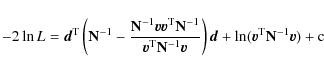
In the past, marginalization over systematic parameters has been
carried out either numerically or analytically (Bridle et al. 2002); both methods are currently implemented in cosmomc (Lewis & Bridle 2002). Assuming likelihoods are Gaussian one typically has a marginalization of the form:
![\begin{displaymath}%
L \propto \int {\rm d} \alpha P(\alpha) \exp [ -(\alpha {\v...
...\vec d})^{\rm T} {\bf N}^{-1} (\alpha {\vec v}- {\vec d}) /2 ]
\end{displaymath}](/articles/aa/full_html/2010/05/aa13032-09/img20.png)
|
(1) |
where
|
(2) |
where
|
(3) |
In the case of beam uncertainties, the analytic approach is feasible only if the beams are assumed to be Gaussian. This is not realistic.
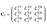
It is customary to characterize anisotropies in the Cosmic Microwave Background by their angular power spectrum,
![]() for both temperature and polarization.
for both temperature and polarization.
![]() is a 3
is a 3 ![]() 3 matrix for T (temperature) and E or B (grad-type or curl-type polarization):
3 matrix for T (temperature) and E or B (grad-type or curl-type polarization):
|
(4) |
Hereafter, for the sake of simplicity, most equations will refer to the angular power spectrum,
To obtain unbiased estimates of the parameters that characterize the cosmology, we must repair this suppression based on knowledge of the beam. Uncertainties in the beam propagate into uncertainties in the cosmological parameters.
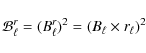
We assume that the beam uncertainties can be described by a set
of functions or templates, taken here to be the set of transfer
functions obtained by the beam fitting procedure described in
Sect. 3. These templates are given in multipole space by:
|
(5) |
where the ratios
To estimate constraints on cosmological parameters, we need to
compare the model with the data via a chosen Likelihood and an
algorithm to sample cosmological parameters. Here we make use of the
package cosmomc. To incorporate MCBR we modify cosmomc to enable the usage of a random
![]() for each theoretical model generated with CAMB (Lewis et al. 2000) or PICO (Fendt & Wandelt 2006).
This is done by modifying the cmbdata module of the cosmomc code.
for each theoretical model generated with CAMB (Lewis et al. 2000) or PICO (Fendt & Wandelt 2006).
This is done by modifying the cmbdata module of the cosmomc code.
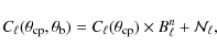
We start by creating simulated datasets with noise properties specific
to the instrument under consideration, in our case Planck and an
example of a future experiment (see Sect. 4). These simulated datasets are given in terms of the angular Power Spectrum
![]() :
:
where
![\begin{figure}
\par\includegraphics[width=12cm,clip]{figure/13032fg1.ps}
\vspace*{5mm}
\end{figure}](/articles/aa/full_html/2010/05/aa13032-09/img44.png)
|
Figure 1:
Marginalized parameter constraints for Planck 143 GHz with 7' beam with |
| Open with DEXTER | |
As our purpose here is to introduce and validate the MCBR
method it suffices to assume full-sky coverage. Considerations of
realistic complications (such as cut-sky, foregrounds, etc.)
is deferred to a future publication. Our purpose here is to
establish the relative importance of propagating beam errors to
cosmological parameters rather than to make comprehensive predictions
for Planck. Hereafter to compare the observed dataset,
![]() ,
with theoretical models we use the exact full-sky likelihood (with
,
with theoretical models we use the exact full-sky likelihood (with
![]() )
(Bond et al. 2000):
)
(Bond et al. 2000):
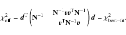
i.e., the Inverse Wishart distribution for Temperature and Polarization. In cosmomc this distribution is coded in function ChiSqExact (Lewis 2005). We analyse these datasets with a modified version of this function, built to include the MCBR procedure in the code.
The ![]() of the theoretical model is given by:
of the theoretical model is given by:

where
where
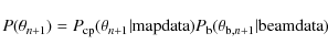
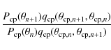
In the MCBR scheme, sampling of the beam templates is
equivalent to sampling from the proposal distribution. The
Metropolis-Hastings algorithm accepts the move from
![]() to
to
![]() in the Markov chain by evaluating the ratio:
in the Markov chain by evaluating the ratio:
where P is the posterior distribution we wish to sample from and q is the proposal distribution. We draw the proposal at position
|
(12) |
where
| (13) |
Furthermore
|
(14) |
(for instance in our study here
|
(15) |
as
Hence random sampling from the set of beam templates at each step of the Markov chain is equivalent to sampling from a proposal density that, by construction, is identical to the posterior distribution of the beam parameters given the beam fitting data.
To illustrate how the MCBR procedure works, we give here the steps followed in our analysis (see Sect. 5). We start by comparing two cases:
- 1.
- cosmomc run with the ``true'' fiducial beam transfer alone,
 ;
;
- 2.
- cosmomc run with the MCBR procedure for the set of beam transfer functions,
 ,
obtained from the beam fitting step.
,
obtained from the beam fitting step.
- we generate a simulated data set using as fiducial the ``true'' beam transfer
;
- we analyse this simulated data set with cosmomc, including in the code just the effect of the
(i.e. the theoretical
 is multiplied by the true beam transfer,
);
is multiplied by the true beam transfer,
);
- we analyse this simulated data set with a modified version of cosmomc in which the theoretical
is multiplied by the randomly chosen beam,
at each step of the chain - i.e., with in-built MCBR
2.1 Validation
To demonstrate that that the MCBR technique gives correct marginalized errors, we compared the results given by MCBR to those from a ``brute force'' cosmomc
calculation in which the beam was taken as another parameter. We did
this for three simulated datasets, the first generated using the
``true'' beam transfer function
![]() ,
the second and third using beam transfer functions that were
chosen to be mildly and extremely far from the true one,
respectively. We simplified the test cases by assuming that the beam
was a symmetric 7' (FWHM) Gaussian, with 4% variations of the fwhm of the beam.
,
the second and third using beam transfer functions that were
chosen to be mildly and extremely far from the true one,
respectively. We simplified the test cases by assuming that the beam
was a symmetric 7' (FWHM) Gaussian, with 4% variations of the fwhm of the beam.
The brute force calculation was done by probing the beam parameter space in cosmomc in the same way as for any of the other parameters, and considering the default proposal density already implemented in cosmomc. The beam parameter is included by transforming the theoretical
![]() output by CAMB at each Markov chain step into
output by CAMB at each Markov chain step into
|
(16) |
where
![\begin{figure}
\par\includegraphics[width=12cm,clip]{figure/13032fg2.ps}
\vspace*{6.5mm}
\end{figure}](/articles/aa/full_html/2010/05/aa13032-09/img83.png)
|
Figure 2:
Marginalized parameter constraints for Planck 143 GHz with 7' beam with |
| Open with DEXTER | |
![\begin{figure}
\par\includegraphics[width=12cm,clip]{figure/13032fg3.ps}
\vspace*{6.5mm}
\end{figure}](/articles/aa/full_html/2010/05/aa13032-09/img84.png)
|
Figure 3:
Marginalized parameter constraints for Planck 143 GHz with 7' beam with |
| Open with DEXTER | |
For the MCBR calculation we analysed the simulated data with a modified version of cosmomc in which the theoretical ![]() is multiplied by the randomly chosen beam transfer,
is multiplied by the randomly chosen beam transfer,
![]() at each step of the chain.
at each step of the chain.
The results are plotted in Figs. 1-3.
In all cases, we find same parameter distributions for both
methods. As expected, the extreme deviated beam results in a
biased estimation of parameters, especially ![]() ,
but equally for both the ``beamparameter'' and the MCBR procedures.
,
but equally for both the ``beamparameter'' and the MCBR procedures.
![\begin{figure}
\par\includegraphics[width=8.6cm,clip]{figure/13032fg4a.eps}\hspa...
...cludegraphics[width=8.6cm,clip]{figure/13032fg4b.eps}
\vspace*{5mm}
\end{figure}](/articles/aa/full_html/2010/05/aa13032-09/img85.png)
|
Figure 4:
At each multipole, |
| Open with DEXTER | |
3 Beam fits and transfer function ensembles
We characterize the beam uncertainty for Planck with a Monte Carlo ensemble of transfer functions (Huffenberger et al. 2010) generated by repeated simulation of Jupiter observations using the detector noise and pointing errors expected before flight. Each realization yields a representative transfer function. The beams are calculated with GRASP9 (Sandri et al. 2002, 2010, in prep.; Maffei et al. 2010, in prep.; Yurchenko et al. Yurchenko et al. 2004), and we employ two methods of beam reconstruction to reproduce them from the planet scans. The first uses a rigid linearized parametric model; the second expands the beam in orthogonal functions (see Rocha et al. 2001, for a previous application of such functions in CMB analysis). Figure 5 shows the nominal Gaussian beams with blue-book fwhm values to that of the fiducial realistic Grasp beams based on a Gaussian fit (see Table 1). From the beam reconstruction procedure presented in Huffenberger et al. (2010) we obtain the ratio of the power spectrum as corrected with the fitted beam to the power spectrum as it should have been corrected by the true beam. In Fig. 4 we display lines which bound 68% of the ensemble transfer functions for Planck channels.
Table 1:
Planck (Planck Blue Book 2005) and Epic (Bock et al. 2008) experimental specifications![]() .
.
The simulation of repeated Jupiter calibrations is done in such way that each template is an unbiased estimator of the true template. But in real life, they could be a biased estimator (for instance the Planck pointing error could bias the beam function always in the same direction). This prompted us to consider the runs presented in Sect. 5.2.
The Beam fitting is applied to data with white + 1/f noise,
and to destriped data, i.e., after application e.g. of
a ``destriping'' mapmaking code which removes almost all of the
effects of 1/f noise (Poutanen et al. 2006; Ashdown et al. 2007a,b, 2009).
We use realistic Grasp beams and the parametric model of the
reconstructed beams (the results with non-parametric model will be
presented in a future paper). Figure 6
shows extreme and mild beam transfer functions for the Planck
70 GHz, 100 GHz, 143 GHz and 217 GHz channels
obtained from the beam fitting procedure applied to destriped data
(hence containing a a very low level of 1/f residuals). For comparison purposes we plot in Fig. 7 these functions obtained from data with a white and 1/f noise background.
We also plot in Figs. 8 the normalized histograms of the ratios,
![]() ,
for singe multipoles
,
for singe multipoles
![]() .
For all channels the distributions are slightly skewed and get broader with increasing multipole
.
For all channels the distributions are slightly skewed and get broader with increasing multipole ![]() for each channel. We can also compare the probability of the mildly
deviated and extremely deviated transfer functions used in Sect. 5. For instance for 70 GHz for
for each channel. We can also compare the probability of the mildly
deviated and extremely deviated transfer functions used in Sect. 5. For instance for 70 GHz for ![]() the mild function is
the mild function is
![]() probable while the extreme function is approximately 100 times
less likely. The maximum variation for transfer function ratios,
probable while the extreme function is approximately 100 times
less likely. The maximum variation for transfer function ratios,
![]() ,
is of the order
,
is of the order ![]() for 70 GHz (
for 70 GHz (![]() for 100 GHz) for destriped data, while for white and 1/f noise data with no attempt at destriping it increases to
for 100 GHz) for destriped data, while for white and 1/f noise data with no attempt at destriping it increases to
![]() for the 70 GHz channel (
for the 70 GHz channel (
![]() for 100 GHz).
for 100 GHz).
![\begin{figure}
\par\includegraphics[width=8.5cm,clip]{figure/13032fg5.ps}
\vspace*{5mm}
\end{figure}](/articles/aa/full_html/2010/05/aa13032-09/img96.png)
|
Figure 5: Nominal Gaussian blue-book beams (dotted line) vs. Fiducial realistic Grasp9 beams based on a Gaussian fit (solid line) for 70 GHz (black), 100 GHz (red), 143 GHz (green) and 217 GHz (blue). |
| Open with DEXTER | |
![\begin{figure}
\par\includegraphics[width=9cm,height=5.5cm]{figure/13032fg6a.ps}...
...graphics[width=9cm,height=5.5cm]{figure/13032fg6b.ps}
\vspace*{5mm}
\end{figure}](/articles/aa/full_html/2010/05/aa13032-09/img97.png)
|
Figure 6: Extreme ( left) and Mild ( right) beam transfer functions for the Planck 70 GHz (black), 100 GHz (red), 143 GHz (green) and 217 GHz (blue) channels obtained from beam fitting applied to destriped data. |
| Open with DEXTER | |
![\begin{figure}
\par\includegraphics[width=9cm,height=5.5cm]{figure/13032fg7a.ps}...
...graphics[width=9cm,height=5.5cm]{figure/13032fg7b.ps}
\vspace*{5mm}
\end{figure}](/articles/aa/full_html/2010/05/aa13032-09/img98.png)
|
Figure 7: Extreme ( left) and Mild ( right) beam transfer functions for the Planck 70 GHz (black), 100 GHz (red), 143 GHz (green) and 217 GHz (blue) channels obtained from beam fitting applied to data with white + 1/f noise. |
| Open with DEXTER | |
![\begin{figure}
\par\includegraphics[width=9cm,clip]{figure/13032fg8.ps}
\vspace*{3mm}
\end{figure}](/articles/aa/full_html/2010/05/aa13032-09/img99.png)
|
Figure 8:
Normalized distributions of the beam transfer functions,
|
| Open with DEXTER | |
![\begin{figure}
\par\includegraphics[width=8.7cm,clip]{figure/13032fg9.ps}
\end{figure}](/articles/aa/full_html/2010/05/aa13032-09/img100.png)
|
Figure 9: CMB angular power spectrum (best fit of WMAP 1 yr, black line) and noise levels for Planck: 70 GHz (black), 100 GHz (red), 143 GHz (green), 217 GHz (blue) and for Epic 150 GHz (cian). |
| Open with DEXTER | |
In Sect. 5 we infer that the parameter constraints from beams obtained with destriped data are slightly worse but very close to those obtained with a white noise background as expected.
![\begin{figure}
\par\includegraphics[width=12cm,clip]{figure/13032fg10.ps}
\end{figure}](/articles/aa/full_html/2010/05/aa13032-09/img101.png)
|
Figure 10: Marginalized parameter constraints for Planck 70 GHz without beam uncertainty (black), marginalized over the beam uncertainty via MCBR considering the destriped data (red), and in the presence of white noise + 1/f noise (blue). |
| Open with DEXTER | |
![\begin{figure}
\par\includegraphics[width=12cm,clip]{figure/13032fg11.ps}
\end{figure}](/articles/aa/full_html/2010/05/aa13032-09/img102.png)
|
Figure 11: Marginalized parameter constraints for Planck 100 GHz without beam uncertainty (black), marginalized over the beam uncertainty via MCBR considering the destriped data (red) and in the presence of white noise + 1/f noise (blue). |
| Open with DEXTER | |
4 Analysis: from Beam transfer function uncertainties to parameter estimation
To propagate the beam measurement errors to parameters we apply the MCBR method following the procedure described in Sect. 2. We make use of the beam transfer functions obtained with the beam fitting described in Sect. 3. For this purpose we use a modified version of cosmomc with built-in MCBR step as described in Sect. 2.
We consider a set of five chains. The convergence diagnostic is based
on the Gelman and Rubin statistic, as usual in the field.
Following MCBR, we choose randomly the beam transfer function
(from the set of 1280 simulations) for each step of the
markov chain. We sample a six-dimensional set of cosmological
parameters, with flat priors: the physical baryon and Cold Dark Matter
densities,
![]() and
and
![]() ;
the ratio of the sound horizon to the angular diameter distance at decoupling,
;
the ratio of the sound horizon to the angular diameter distance at decoupling,
![]() ;
the scalar spectral index
;
the scalar spectral index ![]() ;
the overall normalization of the spectrum
;
the overall normalization of the spectrum
![]() at k=0.05 Mpc-1 (hereafter
at k=0.05 Mpc-1 (hereafter ![]() ), and the optical depth to reionization
), and the optical depth to reionization ![]() .
We use a cosmic age top-hat prior 10 Gyr
.
We use a cosmic age top-hat prior 10 Gyr
![]() 20 Gyr, consider purely adiabatic initial conditions only, we
impose flatness, and we treat the dark energy component as a
cosmological constant.
20 Gyr, consider purely adiabatic initial conditions only, we
impose flatness, and we treat the dark energy component as a
cosmological constant.
We create simulated datasets with the noise properties of the Planck 70, 100, 143 and 217 GHz (Planck Blue Book 2005)
channels, as well as one example of a future experiment. For the latter
we considered the noise levels of Epic 150 GHz (Bock et al. 2008). We take as our cosmological model the best fit of WMAP 1 yr:
![]() ;
;
![]() ;
H0 = 71.992;
;
H0 = 71.992;
![]() ;
;
![]() ;
and
;
and
![]() (Spergel et al. 2003). These simulated datasets are given in terms of the angular Power Spectrum
(Spergel et al. 2003). These simulated datasets are given in terms of the angular Power Spectrum
![]() as described in Sect. 2. We compute the noise
as described in Sect. 2. We compute the noise
![]() for Planck and Epic from the sensitivity
for Planck and Epic from the sensitivity
![]() and the nominal
and the nominal ![]() of the beam assuming a Gaussian profile (tabulated in Table 1). In Fig. 9
we plot the theoretical model vs. the noise levels for each
channel considered. Results from this analysis are given in Sect. 5.
of the beam assuming a Gaussian profile (tabulated in Table 1). In Fig. 9
we plot the theoretical model vs. the noise levels for each
channel considered. Results from this analysis are given in Sect. 5.
![\begin{figure}
\par\includegraphics[width=12cm,clip]{figure/13032fg12.ps}
\vspace*{7.5mm}
\end{figure}](/articles/aa/full_html/2010/05/aa13032-09/img118.png)
|
Figure 12: Marginalized parameter constraints for Planck 143 GHz without beam uncertainty (black), marginalized over the beam uncertainty MCBR considering the destriped data (red) and in the presence of white noise + 1/f noise (blue). |
| Open with DEXTER | |
![\begin{figure}
\par\includegraphics[width=12cm,clip]{figure/13032fg13.ps}
\vspace*{7.5mm}
\end{figure}](/articles/aa/full_html/2010/05/aa13032-09/img119.png)
|
Figure 13: Marginalized parameter constraints for Planck 217 GHz without beam uncertainty (black), marginalized over the beam uncertainty MCBR considering the destriped data (red) and in the presence of white noise + 1/f noise (blue). |
| Open with DEXTER | |
Table 2:
Mean values and marginalized ![]() c.l. limits using the fiducial beam: analysis without beam uncertainty
(Col. 3), accounting the beam uncertainty from destriped data
(Col. 4) and from the data with white and 1/f noise (Col. 5).
c.l. limits using the fiducial beam: analysis without beam uncertainty
(Col. 3), accounting the beam uncertainty from destriped data
(Col. 4) and from the data with white and 1/f noise (Col. 5).
![\begin{figure}
\par\includegraphics[height=5.25cm,width=12cm,clip]{figure/13032fg14.ps}
\vspace*{6.8mm}
\end{figure}](/articles/aa/full_html/2010/05/aa13032-09/img182.png)
|
Figure 14:
Marginalized constraints for the most impacted parameters, |
| Open with DEXTER | |
5 Results
5.1 Results: effect of beam uncertainties
Figures 10-13
show the marginalized parameter constraints for Planck in three cases:
without beam uncertainty (i.e., considering the true fiducial beam)
(black); with beam uncertainty using the beam transfer functions
obtained using the destriped data (red); and in the presence of 1/f noise (blue). Table 2 gives the input cosmological parameters and the mean values and marginalized ![]() confidence limits obtained after accounting for the beam errors. To facilitate comparisons, Fig. 14 shows these same marginalized constraints for
confidence limits obtained after accounting for the beam errors. To facilitate comparisons, Fig. 14 shows these same marginalized constraints for ![]() and
and ![]() ,
the parameters where the largest differences are seen between the three cases.
,
the parameters where the largest differences are seen between the three cases.
Equivalent results for a more sensitive polarization experiment - Epic 150 GHz - are plotted in Fig. 15; corresponding parameter values are given in Table 2.
![\begin{figure}
\par\includegraphics[width=12cm,clip]{figure/13032fg15.ps}
\vspace*{7mm}
\end{figure}](/articles/aa/full_html/2010/05/aa13032-09/img183.png)
|
Figure 15: Marginalized parameter constraints for a future experiment with Epic 150 GHz specifications without beam uncertainty (black), marginalized over the beam uncertainty considering the destriped data (red) and in the presence of white noise + 1/f noise (blue). |
| Open with DEXTER | |
The most noticeable effect of beam uncertainties is to widen the marginal distributions of some parameters, especially ![]() ,
for uncertainties obtained in the presence of 1/f noise but without destriping.
,
for uncertainties obtained in the presence of 1/f noise but without destriping. ![]() , and
, and
![]() are also affected. In this case the distribution of the fitted
beam transfer functions is wider than that obtained from white noise or
destriped data as shown in Figs. 6 and 7.
are also affected. In this case the distribution of the fitted
beam transfer functions is wider than that obtained from white noise or
destriped data as shown in Figs. 6 and 7.
Define
![]() ,
the width of the distribution when beam errors are marginalised by applying MCBR, and
,
the width of the distribution when beam errors are marginalised by applying MCBR, and
![]() ,
the width of the distribution for the simulated data convolved with the
fiducial beam (with no beam errors included). Figure 16 shows the enhancement factor,
,
the width of the distribution for the simulated data convolved with the
fiducial beam (with no beam errors included). Figure 16 shows the enhancement factor,
![]() ,
for parameters
,
for parameters ![]() and
and ![]() for beams fitted on data with white + 1/f noise. For example, at 100 GHz the distributions of
for beams fitted on data with white + 1/f noise. For example, at 100 GHz the distributions of ![]() and
and ![]() widen by 25% and 11%, respectively.
widen by 25% and 11%, respectively.
This widening is much reduced by the use of destriping techniques. For
example, with destriping the uncertainties in the beams are 0.5%
for 100 GHz at ![]() ,
which translates into an increase of parameter uncertainties of 0.1%. Without destriping, the uncertainties on
,
which translates into an increase of parameter uncertainties of 0.1%. Without destriping, the uncertainties on ![]() at 70 GHz and on
at 70 GHz and on ![]() at 100 GHz increase by 21% and 25%, respectively, for beams fitted on white + 1/f noise
data. This is a convincing demonstration of the relevance and power of
destriping techniques in reducing the effect of 1/f noise for Planck.
at 100 GHz increase by 21% and 25%, respectively, for beams fitted on white + 1/f noise
data. This is a convincing demonstration of the relevance and power of
destriping techniques in reducing the effect of 1/f noise for Planck.
5.2 Results: effect of assuming a wrong fiducial beam
To illustrate the effect of incorrect beam assumptions we calculated
parameters assuming a mildly and then an extremely ``wrong'' beam.
Specifically, we generated three simulated datasets, using:
![]() ;
a mildly wrong beam
;
a mildly wrong beam
![]() ;
and an extremely wrong beam
;
and an extremely wrong beam
![]() .
We analyzed these datasets with the modified version of cosmomc with MCBR built in, and compared the cosmological parameters from the run with for the ``true'' fiducial beam
.
We analyzed these datasets with the modified version of cosmomc with MCBR built in, and compared the cosmological parameters from the run with for the ``true'' fiducial beam
![]() to those of both the mild and extreme deviated beams.
to those of both the mild and extreme deviated beams.
![\begin{figure}
\par\includegraphics[width=9cm,clip]{figure/13032fg16.ps}
\vspace*{6mm}
\end{figure}](/articles/aa/full_html/2010/05/aa13032-09/img187.png)
|
Figure 16:
Enhancement factor,
|
| Open with DEXTER | |
Table 3:
Bias on ![]() and
and ![]() in units of the error due to the deviation of the extreme function
in units of the error due to the deviation of the extreme function
![]() at
at
![]() ,
after MCBR, fitted on destriped data. For each Planck channel.
,
after MCBR, fitted on destriped data. For each Planck channel.
Figures 17-20
show marginalized parameter constraints from 70 GHz, 100 GHz,
143 GHz, and 217 GHz, respectively, on destriped data. We see
that assuming an extreme beam deviation in the simulated data results
in a biased estimation of some parameters, particularly ![]() .
This is mostly due to incomplete marginalization, as we do
not encompass an adequate distribution of deviations from the chosen
fitted transfer function.
.
This is mostly due to incomplete marginalization, as we do
not encompass an adequate distribution of deviations from the chosen
fitted transfer function.
For comparison, Figs. 21 and 22 show marginalized parameter constraints for the 100 GHz and 143 GHz channels, respectively, on data that have not been destriped.
![\begin{figure}
\par\includegraphics[width=12cm,clip]{figure/13032fg17.ps}
\end{figure}](/articles/aa/full_html/2010/05/aa13032-09/img189.png)
|
Figure 17: Marginalized parameter constraints for Planck 70 GHz with beam randomization MCBR: true beam (black), decreasing function for destriped data (red), increasing function for destriped data (blue), mild deviation (solid line) and extreme deviation from the true beam (dotted line). |
| Open with DEXTER | |
![\begin{figure}
\par\includegraphics[width=12cm,clip]{figure/13032fg18.ps}
\end{figure}](/articles/aa/full_html/2010/05/aa13032-09/img190.png)
|
Figure 18: Marginalized parameter constraints for Planck 100 GHz with beam randomization MCBR: true beam (black), decreasing function for destriped data (red), increasing function for destriped data (blue), mild deviation (solid line) and extreme deviation from the true beam (dotted line). |
| Open with DEXTER | |
![\begin{figure}
\par\includegraphics[width=12cm,clip]{figure/13032fg19.ps}
\end{figure}](/articles/aa/full_html/2010/05/aa13032-09/img191.png)
|
Figure 19: Marginalized parameter constraints for Planck 143 GHz with beam randomization MCBR: true beam (black), decreasing function for destriped data (red), increasing function for destriped data (blue), mild deviation (solid line) and extreme deviation from the true beam (dotted line). |
| Open with DEXTER | |
![\begin{figure}
\par\includegraphics[width=12cm,clip]{figure/13032fg20.ps}
\end{figure}](/articles/aa/full_html/2010/05/aa13032-09/img192.png)
|
Figure 20: Marginalized parameter constraints for Planck 217 GHz with beam randomization MCBR: true beam (black), decreasing function for destriped data (red), increasing function for destriped data (blue), mild deviation (solid line) and extreme deviation from the true beam (dotted line). |
| Open with DEXTER | |
![\begin{figure}
\par\includegraphics[width=12cm,clip]{figure/13032fg21.ps}
\end{figure}](/articles/aa/full_html/2010/05/aa13032-09/img193.png)
|
Figure 21: Marginalized parameter constraints for Planck 100 GHz with beam randomization MCBR: true beam (black), decreasing function for white +1/f noise (red), increasing function for white +1/f noise (blue), mild deviation (solid line) and extreme deviation from the true beam (dotted line). |
| Open with DEXTER | |
![\begin{figure}
\par\includegraphics[width=11cm,clip]{figure/13032fg22.ps}
\end{figure}](/articles/aa/full_html/2010/05/aa13032-09/img194.png)
|
Figure 22: Marginalized parameter constraints for Planck 143 GHz with beam randomization MCBR: true beam (black), decreasing function for white +1/f noise (red), increasing function for white +1/f noise (blue), mild deviation (solid line) and extreme deviation from the true beam (dotted line). |
| Open with DEXTER | |
![\begin{figure}
\par\includegraphics[width=7.6cm,clip]{figure/13032fg23.ps}
\end{figure}](/articles/aa/full_html/2010/05/aa13032-09/img195.png)
|
Figure 23:
Bias on |
| Open with DEXTER | |
Figure 23 shows the bias in ![]() and
and ![]() as a function of the extreme beams fitted on destriped data. We consider the error on
as a function of the extreme beams fitted on destriped data. We consider the error on ![]() given by
given by
![]() for
for
![]() representing the sigma of the beam. The corresponding values are given in Table 3. For example for 100 GHz an uncertainty of the extreme beam transfer function
representing the sigma of the beam. The corresponding values are given in Table 3. For example for 100 GHz an uncertainty of the extreme beam transfer function
![]() for
for ![]() of
of
![]() bias the likelihood by
bias the likelihood by
![]() and
and
![]() for
for ![]() and
and ![]() respectively. A beam transfer function known up to
respectively. A beam transfer function known up to ![]() will bias
will bias ![]() by
by
![]() .
If we had not taken into account the beam uncertainties, then the
same deviation in the transfer functions would have biased
.
If we had not taken into account the beam uncertainties, then the
same deviation in the transfer functions would have biased ![]() by as much as
by as much as
![]() ,
as can be inferred from Fig. 16. The inadequacy of a likelihood that does not integrate the beam uncertainties is mentioned in (Huffenberger et al. 2010). There a simplified analysis of noisier data (only 1 horn) with all parameters except
,
as can be inferred from Fig. 16. The inadequacy of a likelihood that does not integrate the beam uncertainties is mentioned in (Huffenberger et al. 2010). There a simplified analysis of noisier data (only 1 horn) with all parameters except ![]() fixed indicated that limiting the bias to
fixed indicated that limiting the bias to
![]() would require knowledge of
would require knowledge of
![]() to 0.04% where it has fallen to 1% of peak (
to 0.04% where it has fallen to 1% of peak (
![]() for 100 GHz). In our analysis here we see that at
for 100 GHz). In our analysis here we see that at
![]() an uncertainty of 0.5% for the extreme function would bias
an uncertainty of 0.5% for the extreme function would bias ![]() by
by
![]() ,
while a mild deviation of the order 0.2% would produce a bias below
,
while a mild deviation of the order 0.2% would produce a bias below
![]() (see Table 2). Hence a beam deviation five times that reported in Huffenberger et al. (2010) would bias
(see Table 2). Hence a beam deviation five times that reported in Huffenberger et al. (2010) would bias ![]() by less than
by less than
![]() .
This improvement is mostly due to properly marginalizing over the beam uncertainties via the MCBR method.
.
This improvement is mostly due to properly marginalizing over the beam uncertainties via the MCBR method.
6 Conclusions
We have developed a fast new method, MCBR, to propagate beam uncertainties to parameter estimation. The method properly accounts for the marginalised errors in the parameters. A desirable feature of the method is that it makes minimal assumptions on beam uncertainties. For example, it does not assume the data are normally distributed, and, unlike other approaches such as analytic marginalization, it does not require Gaussian priors on the specific systematic uncertainty. Furthermore it accounts accurately for the shape of the beam as it makes use of beam uncertainty templates for such beams, hence there is no need for simplified a priori assumptions on their shapes. Finally MCBR can be generalized and used to propagate other systematic uncertainties, as long as a set of templates of such systematics is provided.
From the study presented here on propagating the beam measurement errors to parameter estimation via the new MCBR method for Planck and for a future experiment, we conclude:
- Removal of 1/f noise residuals, by destriping or other techniques, is quite important.
- The main impact of beam uncertainties is to widen the marginal distributions of some parameters (most notably
 ).
).
- Assuming as extreme beam deviation in the simulated data results in a biased estimation of some parameters (mainly of )
due to incomplete marginalization.
- The parameters more noticeably impacted by beam uncertainties are: ,
 and
and 
When the beam fitting is performed in destriped data the
uncertainties on the beams for say 100 GHz are at most of the
order of ![]() for
for
![]() which translates into an increase of parameter uncertainties at most of the order of
which translates into an increase of parameter uncertainties at most of the order of ![]() .
Instead the uncertainties on
.
Instead the uncertainties on ![]() at 70 GHz and on
at 70 GHz and on ![]() at 100 GHz increases approximately by
at 100 GHz increases approximately by ![]() and
and ![]() respectively for beams fitted on white + 1/f noise data while it remains unaltered for white noise background alone.
respectively for beams fitted on white + 1/f noise data while it remains unaltered for white noise background alone.
The effect of wrong assumptions on beam parameters will bias the
parameter constraints only for extreme deviations from the true beam
and hence for quite atypical circunstances. Considering the analysis
performed on destriped data, at 100 GHz an uncertainty of the
extreme beam transfer function at ![]() of
of
![]() will bias the likelihood by
will bias the likelihood by
![]() and
and
![]() for
for ![]() and
and ![]() ,
respectively. A beam transfer function known to
,
respectively. A beam transfer function known to ![]() will bias
will bias ![]() by
by
![]() .
If we had not taken into account the beam uncertainties, then the
same deviation in the transfer functions would have biased
.
If we had not taken into account the beam uncertainties, then the
same deviation in the transfer functions would have biased ![]() by as much as
by as much as
![]() .
To limit the bias in
.
To limit the bias in ![]() to less than
to less than
![]() will require a knowledge of a mild deviated beam bl2 to
will require a knowledge of a mild deviated beam bl2 to ![]() where it has fallen to 1 percent. A mild deviated function
gives rise to no observable bias (i.e. at most of the order
where it has fallen to 1 percent. A mild deviated function
gives rise to no observable bias (i.e. at most of the order
![]() ).
).
Therefore we expect only a small impact of beam measurement errors on cosmological parameter estimation as long as the beam fitting is performed on destriped data.
G.R. is grateful to Jeffrey Jewell and Lloyd Knox for insightful discussions. L.P. acknowledges support by ASI contract I/016/07/0 ``COFIS''. K.M.H. receives support from NASA via JPL subcontract 1363745. We gratefully acknowledge support by the NASA Science Mission Directorate via the US Planck Project. The research described in this paper was partially carried out at the Jet propulsion Laboratory, California Institute of Technology, under a contract with NASA. Copyright 2009. All rights reserved.
References
- Ashdown, M. A. J., Baccigalupi, C., Balbi, A., et al. 2007a, A&A, 467, 761 [NASA ADS] [CrossRef] [EDP Sciences] [Google Scholar]
- Ashdown, M. A. J., Baccigalupi, C., Balbi, A., et al. 2007b, A&A, 471, 361 [NASA ADS] [CrossRef] [EDP Sciences] [Google Scholar]
- Ashdown, M. A. J., Baccigalupi, C., Bartlett, J. G., et al. 2009, A&A, 493, 753 [NASA ADS] [CrossRef] [EDP Sciences] [Google Scholar]
- Bock, J., Cooray, A., Hanany, S., et al. 2008, [arXiv:0805.4207] [Google Scholar]
- Bond, J. R., Jaffe, A. H., & Knox, L. 2000, ApJ, 533, 19 [NASA ADS] [CrossRef] [Google Scholar]
- Bridle, S. R., Crittenden, R., Melchiorri, A., et al. 2002, MNRAS, 335, 1193B [NASA ADS] [CrossRef] [Google Scholar]
- Fendt, W. A., & Wandelt, B. D. 2006, ApJ, 654, 2 [NASA ADS] [CrossRef] [Google Scholar]
- Huffenberger, K. M., Crill, B. P., Lange, A. E., et al. 2010, A&A, 510, A58 [NASA ADS] [CrossRef] [EDP Sciences] [Google Scholar]
- Lewis, A. 2005, Phys. Rev. D, 71, 083008 [NASA ADS] [CrossRef] [Google Scholar]
- Lewis, A., & Bridle, S. 2002, Phys. Rev. D, 66, 103511 [NASA ADS] [CrossRef] [Google Scholar]
- Lewis, A., Challinor, A., & Lasenby, A. 2000, ApJ, 538, 473 [NASA ADS] [CrossRef] [Google Scholar]
- Planck Collaboration, Planck Blue Book 2005 [arXiv:astro-ph/0604069] [Google Scholar]
- Poutanen, T., CTP, et al. 2006, A&A, 449, 1311 [NASA ADS] [CrossRef] [EDP Sciences] [Google Scholar]
- Rocha, G., Magueijo, J., Hobson, M., & Lasenby, A. 2001, Phys. Rev. D, 64, 063512 [NASA ADS] [CrossRef] [Google Scholar]
- Sandri, M., Bersanelli, M., Burigana, C., et al. 2002, in Experimental Cosmology at Millimetre Wavelengths, ed. M. de Petris, & M. Gervasi, AIP Conf. Ser., 616, 242 [Google Scholar]
- Spergel, D. N., et al. [WMAP Collaboration] 2003, ApJS, 148, 175 [NASA ADS] [CrossRef] [Google Scholar]
- Yurchenko, V. B., Murphy, J. A., & Lamarre, J.-M. 2004, Proc. SPIE 5487, ed. J. C. Mather, 542 [Google Scholar]
All Tables
Table 1:
Planck (Planck Blue Book 2005) and Epic (Bock et al. 2008) experimental specifications![]() .
.
Table 2:
Mean values and marginalized ![]() c.l. limits using the fiducial beam: analysis without beam uncertainty
(Col. 3), accounting the beam uncertainty from destriped data
(Col. 4) and from the data with white and 1/f noise (Col. 5).
c.l. limits using the fiducial beam: analysis without beam uncertainty
(Col. 3), accounting the beam uncertainty from destriped data
(Col. 4) and from the data with white and 1/f noise (Col. 5).
Table 3:
Bias on ![]() and
and ![]() in units of the error due to the deviation of the extreme function
in units of the error due to the deviation of the extreme function
![]() at
at
![]() ,
after MCBR, fitted on destriped data. For each Planck channel.
,
after MCBR, fitted on destriped data. For each Planck channel.
All Figures
|
|
Figure 1:
Marginalized parameter constraints for Planck 143 GHz with 7' beam with |
| Open with DEXTER | |
| In the text | |
|
|
Figure 2:
Marginalized parameter constraints for Planck 143 GHz with 7' beam with |
| Open with DEXTER | |
| In the text | |
|
|
Figure 3:
Marginalized parameter constraints for Planck 143 GHz with 7' beam with |
| Open with DEXTER | |
| In the text | |
|
|
Figure 4:
At each multipole, |
| Open with DEXTER | |
| In the text | |
|
|
Figure 5: Nominal Gaussian blue-book beams (dotted line) vs. Fiducial realistic Grasp9 beams based on a Gaussian fit (solid line) for 70 GHz (black), 100 GHz (red), 143 GHz (green) and 217 GHz (blue). |
| Open with DEXTER | |
| In the text | |
|
|
Figure 6: Extreme ( left) and Mild ( right) beam transfer functions for the Planck 70 GHz (black), 100 GHz (red), 143 GHz (green) and 217 GHz (blue) channels obtained from beam fitting applied to destriped data. |
| Open with DEXTER | |
| In the text | |
|
|
Figure 7: Extreme ( left) and Mild ( right) beam transfer functions for the Planck 70 GHz (black), 100 GHz (red), 143 GHz (green) and 217 GHz (blue) channels obtained from beam fitting applied to data with white + 1/f noise. |
| Open with DEXTER | |
| In the text | |
|
|
Figure 8:
Normalized distributions of the beam transfer functions,
|
| Open with DEXTER | |
| In the text | |
|
|
Figure 9: CMB angular power spectrum (best fit of WMAP 1 yr, black line) and noise levels for Planck: 70 GHz (black), 100 GHz (red), 143 GHz (green), 217 GHz (blue) and for Epic 150 GHz (cian). |
| Open with DEXTER | |
| In the text | |
|
|
Figure 10: Marginalized parameter constraints for Planck 70 GHz without beam uncertainty (black), marginalized over the beam uncertainty via MCBR considering the destriped data (red), and in the presence of white noise + 1/f noise (blue). |
| Open with DEXTER | |
| In the text | |
|
|
Figure 11: Marginalized parameter constraints for Planck 100 GHz without beam uncertainty (black), marginalized over the beam uncertainty via MCBR considering the destriped data (red) and in the presence of white noise + 1/f noise (blue). |
| Open with DEXTER | |
| In the text | |
|
|
Figure 12: Marginalized parameter constraints for Planck 143 GHz without beam uncertainty (black), marginalized over the beam uncertainty MCBR considering the destriped data (red) and in the presence of white noise + 1/f noise (blue). |
| Open with DEXTER | |
| In the text | |
|
|
Figure 13: Marginalized parameter constraints for Planck 217 GHz without beam uncertainty (black), marginalized over the beam uncertainty MCBR considering the destriped data (red) and in the presence of white noise + 1/f noise (blue). |
| Open with DEXTER | |
| In the text | |
|
|
Figure 14:
Marginalized constraints for the most impacted parameters, |
| Open with DEXTER | |
| In the text | |
|
|
Figure 15: Marginalized parameter constraints for a future experiment with Epic 150 GHz specifications without beam uncertainty (black), marginalized over the beam uncertainty considering the destriped data (red) and in the presence of white noise + 1/f noise (blue). |
| Open with DEXTER | |
| In the text | |
|
|
Figure 16:
Enhancement factor,
|
| Open with DEXTER | |
| In the text | |
|
|
Figure 17: Marginalized parameter constraints for Planck 70 GHz with beam randomization MCBR: true beam (black), decreasing function for destriped data (red), increasing function for destriped data (blue), mild deviation (solid line) and extreme deviation from the true beam (dotted line). |
| Open with DEXTER | |
| In the text | |
|
|
Figure 18: Marginalized parameter constraints for Planck 100 GHz with beam randomization MCBR: true beam (black), decreasing function for destriped data (red), increasing function for destriped data (blue), mild deviation (solid line) and extreme deviation from the true beam (dotted line). |
| Open with DEXTER | |
| In the text | |
|
|
Figure 19: Marginalized parameter constraints for Planck 143 GHz with beam randomization MCBR: true beam (black), decreasing function for destriped data (red), increasing function for destriped data (blue), mild deviation (solid line) and extreme deviation from the true beam (dotted line). |
| Open with DEXTER | |
| In the text | |
|
|
Figure 20: Marginalized parameter constraints for Planck 217 GHz with beam randomization MCBR: true beam (black), decreasing function for destriped data (red), increasing function for destriped data (blue), mild deviation (solid line) and extreme deviation from the true beam (dotted line). |
| Open with DEXTER | |
| In the text | |
|
|
Figure 21: Marginalized parameter constraints for Planck 100 GHz with beam randomization MCBR: true beam (black), decreasing function for white +1/f noise (red), increasing function for white +1/f noise (blue), mild deviation (solid line) and extreme deviation from the true beam (dotted line). |
| Open with DEXTER | |
| In the text | |
|
|
Figure 22: Marginalized parameter constraints for Planck 143 GHz with beam randomization MCBR: true beam (black), decreasing function for white +1/f noise (red), increasing function for white +1/f noise (blue), mild deviation (solid line) and extreme deviation from the true beam (dotted line). |
| Open with DEXTER | |
| In the text | |
|
|
Figure 23:
Bias on |
| Open with DEXTER | |
| In the text | |
Copyright ESO 2010
Current usage metrics show cumulative count of Article Views (full-text article views including HTML views, PDF and ePub downloads, according to the available data) and Abstracts Views on Vision4Press platform.
Data correspond to usage on the plateform after 2015. The current usage metrics is available 48-96 hours after online publication and is updated daily on week days.
Initial download of the metrics may take a while.