| Issue |
A&A
Volume 523, November-December 2010
|
|
|---|---|---|
| Article Number | A72 | |
| Number of page(s) | 18 | |
| Section | Extragalactic astronomy | |
| DOI | https://doi.org/10.1051/0004-6361/200913014 | |
| Published online | 18 November 2010 | |
Magnetised winds in dwarf galaxies
1
Astrophysics, University of Oxford,
Denys Wilkinson Building, Keble Road, Oxford,
OX13,
RH,
UK
e-mail: yohan.dubois@physics.ox.ac.uk
2
Universität Zürich, Institute für Theoretische Physik,
Winterthurerstrasse
190, 8057
Zürich,
Switzerland
3
CEA Saclay, DSM/IRFU/SAP, Bâtiment 709, 91191
Gif-sur-Yvette Cedex,
France
Received:
29
July
2009
Accepted:
7
July
2010
Context. The generation and the amplification of magnetic fields in the current cosmological paradigm are still open questions. The standard theory is based on an early field generation by Biermann battery effects, possibly at the epoch of reionisation, followed by a long period of field amplification by galactic dynamos. The origin and the magnitude of the inter-galactic magnetic field is of primordial importance in this global picture, as it is considered to be the missing link between galactic magnetic fields and cluster magnetic fields on much larger scales.
Aims. We are testing whether dwarf galaxies are good candidates to explain the enrichment of the Inter-Galactic Medium (IGM): after their discs form and trigger galactic dynamos, supernova feedback will launch strong winds, expelling magnetic field lines in the IGM.
Methods. We have performed magneto-hydrodynamics simulations of an isolated dwarf galaxy, which forms self-consistently inside a cooling halo. Using the RAMSES code, we simulated for the first time the formation of a magnetised supernova-driven galactic outflow. This simulation is an important step towards a more realistic modelling using fully cosmological simulations.
Results. Our simulations reproduce well the observed properties of magnetic fields in spiral galaxies. The formation and the evolution of our simulated disc leads to a strong magnetic field amplification: the magnetic field in the final wind bubble is one order of magnitude larger than the initial value. The magnetic field in the disc, essentially toroidal, is growing linearly with time as a consequence of differential rotation.
Conclusions. We discuss the consequence of this simple mechanism on the cosmic evolution of the magnetic field: we propose a new scenario for the evolution of the magnetic field, with dwarf galaxies playing a key role in amplifying and ejecting magnetic energy in the IGM, resulting in what we call a “cosmic dynamo” that could contribute to the very high field strengths observed in galaxies and clusters today.
Key words: galaxies: formation / galaxies: evolution / galaxies: magnetic fields / methods: numerical
© ESO, 2010
1. Introduction
The origin of magnetic fields in the Universe is a long-standing puzzle in cosmology. Although measuring magnetic field in cosmic structures is very challenging, we have strong evidence that magnetic fields exist in many galaxies, with magnitudes between 1 and 10 μG at a level close to equipartition (see the review of Beck et al. 1996). Magnetic fields of the order of several tens of μG are also detected in large galaxy clusters (see Carilli & Taylor 2002 or Govoni & Feretti 2004, and references therein). However, in the very low density intergalactic medium (IGM), magnetic fields still remain undetected on a large scale (Blasi et al. 1999).
From a theoretical point of view, small-scale fluctuating magnetic fields could be generated from quantum effects during the Big Bang (Turner & Widrow 1988 for example). The amplitude and the correlation length of these primordial fields should both be quite small (Grasso & Rubinstein 2001). Magnetic fields greater than a few nG would also have been detected as a specific source of anisotropy in the cosmic microwave background. More extreme scenarios can also be ruled out: for example, a uniform magnetic field greater than 10-1 μG at our epoch would have led to unexpected anisotropies in the expansion of the Universe (Cheng et al. 1994). Note also that the relic of any magnetic field generated in the early universe, if it is greater than 10-7 μG today, would have broken the symmetry between left and right neutrinos (spin transition) during the period of neutrino production (Enqvist et al. 1993; Sciama 1994).
When the first structures collapsed (z ≃ 10), the Biermann battery (see Kulsrud et al. 1997) is believed to have generated magnetic fields from pure collisional microscopic processes. These magnetic fields appear mainly at shocks and ionisation fronts, where the motions of electrons and ions are decoupled, creating small microscopic currents. It was shown that this battery effect can generate magnetic fields of the order of 10-13 μG field in the IGM (Gnedin et al. 2000). More recently, shocks around primordial mini-halos and the associated first generation of massive stars were also considered as important sources of a magnetic field at high redshift (Xu et al. 2008).
In order to reconcile the very low values quoted above with observations, we need strong amplification processes up to the observed level of magnetic field strength in galaxies and clusters. Gravitational contraction of the frozen-in magnetic field will not be sufficient, because we expect in this case that B scales as ρ2/3.
Using cosmological simulations of galaxy cluster formation, it was shown that one could reproduce the observed field magnitude by considering both gravitational contraction and turbulent stirring of the magnetised gas (Roettiger et al. 1999; Dolag et al. 1999, 2002, 2005; Sigl et al. 2004; Brüggen et al. 2005; Subramanian et al. 2006; Asai et al. 2007; Dubois & Teyssier 2008a). In cooling flow clusters, radiative losses are probabily boosting this amplification mechanism even further (Dubois & Teyssier 2008a), as confirmed by recent observations (Carilli & Taylor 2002). When an active galactic nucleus is releasing energy into the intra-cluster medium, a non-cool core develops and the magnetic field within the core is amplified by the jet-induced turbulence (Dubois et al. 2009). The conclusion of this series of papers is that one needs an initial magnetic field of at least 10-5 μG in the IGM to reach μG values in cluster cores. Note that the finite resolution of these numerical experiments probably leads to an underestimation of the turbulent amplification of the magnetic field. Nevertheless, this indirectly justifies very low values for the magnetic field in the IGM, which are still significantly higher than Biermann battery generated fields though.
In order to explain the origin of this diffuse cosmic magnetic field, Bertone et al. (2006) proposed galactic winds as a possible solution to explain the enrichment of the IGM by metals and magnetic fields. In this scenario, magnetic fields are amplified inside galactic discs by the so-called galactic dynamo (Kulsrud 1999), and in a second phase, supernova-driven winds are expelling field lines into the surrounding IGM.
The basic idea of the galactic dynamo (Parker 1971; Ferriere 1992a; Brandenburg et al. 1995; Kulsrud 1999; Shukurov 2004) is that small-scale turbulence (precisely cyclonic motions that could result from supernova explosions, Balsara et al. 2004; Gissinger et al. 2009) in the interstellar medium (ISM) sufficiently modify the small-scale magnetic field to make the large-scale component grow significantly. An additional term ∇ × (αB) is added to the induction equation that represents this dynamo amplification of the field, where α ∝ < u.∇ × u > tensor stands for the cyclonic motions of the gas. If one can correctly approximate the α parameter (Ferriere 1992a,b), it is possible to show that the magnetic field can grow in a few Gyr up to its equipartition value (Ferrière & Schmitt 2000). Note that the dynamo theory works only if the galaxy can loose magnetic helicity (Brandenburg & Subramanian 2005), even though it is still debated that the small scale saturation of the α effect really occurs (Field 1995). Numerical simulations of a very small patch (kpc size) of a galaxy from Gressel et al. (2008) demonstrated that such a fast dynamo occurs if supernova explosions can carry some magnetic helicity from the disc to the hot wind. However, one has to reach a tremendous resolution power (parsec scale) in cosmological situations to provide such a long-term dynamo. Galactic winds have been considered as a nice explanation for suppressing some magnetic helicity from the disc, but no clear demonstration of the effect has been performed in a cosmological context. Another issue with galactic dynamo is that the amplification mechanism is probably too slow, especially if one considers recent magnetic field observations in high-redshift galaxies beyond z = 1 (Bernet et al. 2008). These measurements suggest that magnetic amplification must occur very quickly, in less than 5 Gyr. It is also plausible that a fast growth of the field due to turbulent amplification in the first halos at redshift z > 10 could provide an equipartition field before the first galaxies form (Arshakian et al. 2009). Of course it has to be proven that small scale intense magnetic fields are able to generate this large-scale magnetic field observed in galaxies, for this purpose, alternative theories must be explored.
Parker (1992) first suggested that the production of cosmic rays in supernova remnants could generate stronger buoyancy in the ISM and amplify the magnetic field. Simulations of a cosmic ray pressurised medium have shown that it leads to a rapid growth of magnetic lines if they are strongly diffused in the ISM (Hanasz et al. 2004, 2009a,b). Rees (1987) considered Biermann battery effects occuring at the surface of massive stars. More generally, one can consider any stellar dynamo mechanism as an efficient amplification mechanism inside stars (Brun et al. 2004), followed by the release of this magnetic field into the ISM, thanks to stellar winds or supernova explosions. Although the efficiency of the stellar dynamo is rather uncertain (Brandenburg & Subramanian 2005), and the magnetic energy released into supernova remnants is poorly constrained (Kennel & Coroniti 1984, for the Crab nebula & Helfand et al. 2001 for the Vela nubula), this stellar origin represents a very appealing perspective to explain a fast magnetic field generation in high-redshift galaxies.
Galactic dynamos, or other field generation mechanisms in the ISM, together with galactic winds, should therefore play an important role in the generation of magnetic fields in the IGM. In this respect, it is probably inside dwarf galaxies that this double mechanism occurs: dwarf galaxies are very numerous in the early universe, and they host most of the cosmic material at early times (Bertone et al. 2006; Donnert et al. 2009). Dwarf galaxies are also easily disrupted by galactic winds, in contrast to Milky Way-like galaxies, from which metal and magnetic fields probably never escaped (Dubois & Teyssier 2008b, and references therein). Kronberg et al. (1999) proposed a scenario where primeval galaxies launch strong starbursts that generate a 5 × 10⁻³ μG IG magnetic field. They assume that galactic winds are able to reach Mpc scales and that they substantially amplify the field during the outburst.
Understanding the evolution of magnetic fields in dwarf galaxies is therefore an important goal. Performing magneto-hydrodynamics (MHD) numerical simulations with smoothed-particle hydrodynamics (SPH), Kotarba et al. (2009) studied the amplification of the magnetic field by differential rotation and by the spiral pattern of the gaseous disc. Another step was undertaken by Wang & Abel (2009), who performed MHD numerical simulations with adaptive mesh refinement (AMR) of a dwarf galaxy formed by the collapse of a cooling halo. They studied in detail the gas fragmentation and the magnetic field energy amplification due to turbulent, vortical motions induced by the gravitational instability in the disc. Starting with an initially uniform field of 10-3 μG in the halo, they reached equipartition after only a few rotations. They did not simulate, however, the effect of supernova feedback in driving strong outflows out of the galaxy. Bertone et al. (2006), on the other hand, focussed their study on the effect of galactic winds and how they might enrich the Universe with metals and magnetic fields. They used for that purpose a semi-analytical model, assuming equipartition magnetic fields inside their galactic discs and following the wind’s evolution through cosmic times.
In this paper, our goal is to model the evolution of magnetic fields in a dwarf galaxy together with the formation of a galactic wind, in order to compute the amount of magnetic energy that escapes from the disc. This outgoing magnetic energy flux is the key quantity that we need to estimate the efficiency of IGM enrichment. For that purpose, we simulate an isolated, cooling halo, as in Dubois & Teyssier (2008b) and Wang & Abel (2009), and form a small galactic disc in the halo centre. We numerically solve the ideal MHD equations including self-gravity with standard galaxy formation physics (cooling, heating, star formation, supernova feedback). The main parameter in our study is the starting magnetic field that permeates the initial halo. We therefore vary its strength, assuming a simple but realistic initial field geometry. We will also consider the case of a zero initial magnetic field in the halo, in a model where seed fields are introduced within supernova bubbles, implementing the stellar feedback scenario suggested by Rees (1987) in a way similar to Hanasz et al. (2009b). In Sect. 2 we present the numerical set-up of our simulations, as well as some details in our implementation of galaxy formation physics, and in Sect. 3, we discuss our initial conditions more specifically. In Sects. 4 and 5 we present our results on the magnetic amplification in galactic discs, and in Sect. 6 we show how the IGM can be enriched by magnetised galactic winds. We finally comment on the implications of this work in Sect. 7.
2. Numerical methods
2.1. Gas dynamics with magnetic fields
We use the AMR code RAMSES (Teyssier 2002) to
solve the full set of ideal MHD equations
 using
a Godunov scheme with constrained transport that preserves the divergence of the magnetic
field (Teyssier et al. 2006; Fromang et al. 2006). In the previous system, ρ is the
plasma density, ρu is the plasma momentum,
B is the magnetic field,
E = 0.5ρu2 + Eth + B2/8π
is the total energy and Eth is the thermal energy. This system
of conservation laws is closed using the equation of state (EoS) for an ideal mono-atomic
gas, where the total pressure is given by
Ptot = (γ − 1)Eth + B2/8π,
with γ = 5/3. The MHD solver in the RAMSES code has
been tested using idealised cases, as well as more realistic astrophysical situations in
Fromang et al. (2006). It has been used for the
first time in the cosmological context by Dubois &
Teyssier (2008a) to study the evolution of a cooling flow cluster, for which it
produced results that agree well with previous studies (Dolag et al. 2005; Brüggen et al. 2005).
Because it is based on constrained transport, the magnetic divergence exactly vanishes in
an integral sense: the total magnetic flux across each AMR cell boundary is zero. The
electric field is computed at cell edges, using a 2D Riemann solver, in order to upwind
the edge-centred electric field with respect to the four neighbouring cell states. The
2D Riemann solver is based on a generalisation of the 1D HLLD Riemann solver of Miyoshi & Kusano (2005), assuming a 5-wave
piecewise constant Riemann solution. We also account for self-gravity in the gas and
stellar distribution, assuming a static potential for the dark matter component. The
Poisson equation is solved with isolated boundary conditions, using Dirichlet boundary
conditions given by a multipole approximation of the mass distribution in the box. The
gravitational force is added as a source term in both the momentum and the energy
conservation equations.
using
a Godunov scheme with constrained transport that preserves the divergence of the magnetic
field (Teyssier et al. 2006; Fromang et al. 2006). In the previous system, ρ is the
plasma density, ρu is the plasma momentum,
B is the magnetic field,
E = 0.5ρu2 + Eth + B2/8π
is the total energy and Eth is the thermal energy. This system
of conservation laws is closed using the equation of state (EoS) for an ideal mono-atomic
gas, where the total pressure is given by
Ptot = (γ − 1)Eth + B2/8π,
with γ = 5/3. The MHD solver in the RAMSES code has
been tested using idealised cases, as well as more realistic astrophysical situations in
Fromang et al. (2006). It has been used for the
first time in the cosmological context by Dubois &
Teyssier (2008a) to study the evolution of a cooling flow cluster, for which it
produced results that agree well with previous studies (Dolag et al. 2005; Brüggen et al. 2005).
Because it is based on constrained transport, the magnetic divergence exactly vanishes in
an integral sense: the total magnetic flux across each AMR cell boundary is zero. The
electric field is computed at cell edges, using a 2D Riemann solver, in order to upwind
the edge-centred electric field with respect to the four neighbouring cell states. The
2D Riemann solver is based on a generalisation of the 1D HLLD Riemann solver of Miyoshi & Kusano (2005), assuming a 5-wave
piecewise constant Riemann solution. We also account for self-gravity in the gas and
stellar distribution, assuming a static potential for the dark matter component. The
Poisson equation is solved with isolated boundary conditions, using Dirichlet boundary
conditions given by a multipole approximation of the mass distribution in the box. The
gravitational force is added as a source term in both the momentum and the energy
conservation equations.
2.2. Cooling, star formation, and supernova feedback
In order to describe the formation and evolution of a galactic disc, we model gas cooling in the halo as well as in the star-forming disc using a look-up table for the metallicity-dependent radiative cooling function of Sutherland & Dopita (1993) for a mono-atomic gas of H and He with a standard metal mixture. This cooling function is added as a sink term in the energy Eq. (3). The metal mass fraction is advected as a passive scalar, with a source term coming from supernova explosions in the simulated ISM.
Gas is not allowed to cool down to arbitrarily small temperatures. Following the general ideas presented in Yepes et al. (1997) and in Springel & Hernquist (2003), we use a density-dependent temperature floor to account for the unresolved turbulence in the ISM, modelling this complex multiphase medium with an effective EoS. In this paper, we use the following temperature floor Tmin = T0(n/n0)2/3, where n0 is the star-formation density threshold (see below) and T0 = 104 K. The effect of this temperature floor is to prevent the gas from fragmenting down to parsec scales, well below our resolution limit. This is different from the study presented by Wang & Abel (2009), where the gas temperature was allowed to cool down to 300 K, triggering strong disc fragmentation and massive clump formation.
Star formation is implemented using a standard approach based on the Schmidt law, spawning star particles as a random Poisson process. We refer the reader to Rasera & Teyssier (2006) and Dubois & Teyssier (2008b) for more details. We choose here the following star-formation parameters: an efficiency of 5% per free-fall-time and a star-formation density threshold of n0 = 0.1 H.cm-3. Each stellar particle represents a single stellar population of a total mass m∗ = n0mHΔx3 ≃ 104 M⊙. This stellar particle should therefore be considered as a stellar cluster (SC) rather than as an individual star.
After several Myr, the first massive stars explode in supernovae (SN), giving rise to huge expanding bubbles and ultimately to the formation of a large-scale galactic wind. A mass fraction of ηSN = 10% in massive stars M > 8 M⊙ (taken from any standard initial mass function, e.g. Kroupa 2001) is considered for our stellar clusters. Modelling supernova feedback is a delicate numerical issue that crucially depends on the adopted spatial resolution. It was shown by Ceverino & Klypin (2009) that modelling feedback with a pure thermal dump of energy only works at a resolution smaller than 50 pc for a clumpy interstellar medium. We here used a physical size of 150 pc for our smallest cells. We therefore need to rely on a more sophisticated approach to properly model the formation of supernova-driven bubbles. We adopt the now standard kinetic feedback scheme, proposed by various authors (Springel & Hernquist 2003; Dubois & Teyssier 2008b; Dalla Vecchia & Schaye 2008). For each stellar particle formed, we also form an additional collisionless particle in the parent gaseous cell, mimicking the formation of a companion molecular cloud (MC). The mass of the MC is parametrized by mMC = ηwm∗. The free parameter ηw, similar to the one defined in Springel & Hernquist (2003), Rasera & Teyssier (2006) and Dalla Vecchia & Schaye (2008), was chosen to be ηw = 2.
We assume here that after a delay of tSN = 10 Myr, supernova feedback destroys the MC, and that the corresponding mass, momentum, energy, and metal content are released into the surrounding gas cells. Following Dubois & Teyssier (2008b), we add a Sedov blast wave profile to each fluid element for the density, momentum, and total energy, with a radius equal to a fixed physical scale of rSN = 300 pc, or 2 AMR cells. For metal enrichment, we assume a constant yield of ySN = 10% for any exploding star. A stellar cluster with a mass m∗ = 104 M⊙ and zero initial metallicity will release ySNηSNm∗ = 102 M⊙ of metals into the ISM.
When we form a stellar cluster, we do not remove any large-scale magnetic field component. We assume that at small scales the magnetic field is expelled from the collapsing MC by ambipolar diffusion, so that we can neglect the magnetic field that is trapped into the newly formed stars. Similarly, when supernova-driven blast waves form, we do not modify the magnetic field in their surroundings. The magnetic field evolution is therefore driven only by the large-scale velocity field. In only one case do we consider supernova seed fields, as explained in the appendix, in order to test the stellar magnetic feedback scenario proposed by Rees (1987).
3. Initial and boundary conditions
In this section, we describe our initial conditions, especially our initial magnetic topology. We also describe in detail how we enforce the magnetic divergence-free condition at the boundary of the computational domain.
3.1. Initial hydrostatic halo structure
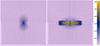 |
Fig. 1 (Oyz) slice of the initial magnetic field amplitude in log μG units and magnetic vectors for BIGM = 10-5 μG at t = 0 Gyr (left pannel) and t = 3 Gyr (right pannel). The picture size is 40 kpc. |
We use the same set of initial conditions as the one presented in Dubois & Teyssier (2008b), namely an isolated dark matter halo
hosting a cooling gaseous component. This idealised situation has been used many times to
study various aspects of galaxy formation (Springel
& Hernquist 2003; Dubois &
Teyssier 2008b; Kaufmann et al. 2009). Let
us recall here only the most important aspects. Dark matter is modelled with a static
density-distribution following a NFW (Navarro et al.
1996) profile in a way that
 (5)where
ρs and
rs are the characteristic density and
radius. This profile can also be parametrized in terms of concentration
c = r200/rs
and virial mass as
(5)where
ρs and
rs are the characteristic density and
radius. This profile can also be parametrized in terms of concentration
c = r200/rs
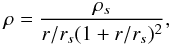
and virial mass as 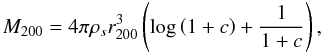 (6)within the virial radius
r200. The virial mass is defined here at an overdensity
equal to 200 times the critical density
ρc. We also assume
H0 = 70 kms-1/Mpc.
(6)within the virial radius
r200. The virial mass is defined here at an overdensity
equal to 200 times the critical density
ρc. We also assume
H0 = 70 kms-1/Mpc.
The gas is initially in hydrostatic equilibrium with the same profile as dark matter,
with a total gas fraction of fb = 15%. We
consider that the halo is slowly rotating, with an angular momentum distribution
consistent with the average specific angular momentum profile measured in cosmological
simulations (Bullock et al. 2001) 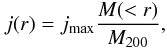 (7)with a spin
parameter
(7)with a spin
parameter 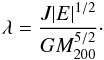 (8)Using this particular
setting, Springel & Hernquist (2003) and
Dubois & Teyssier (2008b) showed that
large-scale outflows are produced only in low-mass halos with
M200 ≲ 1011 M⊙.
As we are interested in the role of galactic winds in the enrichment of the IGM, we
consider here only the case of a small-mass halo with
M200 = 1010 M⊙.
The halo spin parameter is chosen to be λ = 0.1.
(8)Using this particular
setting, Springel & Hernquist (2003) and
Dubois & Teyssier (2008b) showed that
large-scale outflows are produced only in low-mass halos with
M200 ≲ 1011 M⊙.
As we are interested in the role of galactic winds in the enrichment of the IGM, we
consider here only the case of a small-mass halo with
M200 = 1010 M⊙.
The halo spin parameter is chosen to be λ = 0.1.
The box size is set equal to three times the virial radius or L = 150.7 kpc, and is covered by a coarse grid with 643 cells. We consider four additional levels of refinement, so that our effective resolution reaches 10243 or Δx = 147 pc. Our refinement strategy is based on two criteria. First, we refine a cell if its mass exceeds eight times our mass resolution indicator mres = 2 × 10⁻⁶ M200. Second, we refine a cell if the local Jeans length falls below four cells, so that we prevent the disc from artificially fragmenting (Truelove et al. 1997; Bate & Burkert 1997; Machacek et al. 2001). The initial AMR grid was built from the coarse mesh with this refinement strategy. We start initially with a total ~2 × 10⁶ cells, which number remains roughly constant with time. The number of cells in the maximum level of refinement (mainly located in the gaseous disc) is ~4 × 10⁴. After 3 Gyr the total number of stars is ~105.
3.2. Initial magnetic field
Although the choice of the initial magnetic field is very crucial, the magnetic field
topology is usually chosen quite arbitrarily in the literature. Using an initial set-up
very similar to the one presented here, Wang &
Abel (2009) considered a constant initial magnetic field
Bz = 10-9 G. If the initial
halo field is the product of the collapse of some large scale cosmological structure, the
field should preferably scale as  . This scaling
has been observed in cluster-size halos in cosmological MHD simulations (Sigl et al. 2004; Dolag
et al. 2005; Brüggen et al. 2005; Dubois & Teyssier 2008a). In the spherically
symmetric set-up we are considering, each collapsing gas shell will compress and
significantly amplify the frozen-in field, before any disc-like dynamo comes into play.
The initial magnetic field amplitude profile is therefore very important.
In a different context, Kotarba et al. (2009)
considered the case of a pre-existing galactic disc. The initial magnetic field was also
constant, but this time Bx = constant, the
field lines lying exactly in the disc plane. As argued by these authors, differential
rotation quickly takes over and creates a strong toroidal field in the star-forming disc,
so that the initial topology is quickly forgotten.
. This scaling
has been observed in cluster-size halos in cosmological MHD simulations (Sigl et al. 2004; Dolag
et al. 2005; Brüggen et al. 2005; Dubois & Teyssier 2008a). In the spherically
symmetric set-up we are considering, each collapsing gas shell will compress and
significantly amplify the frozen-in field, before any disc-like dynamo comes into play.
The initial magnetic field amplitude profile is therefore very important.
In a different context, Kotarba et al. (2009)
considered the case of a pre-existing galactic disc. The initial magnetic field was also
constant, but this time Bx = constant, the
field lines lying exactly in the disc plane. As argued by these authors, differential
rotation quickly takes over and creates a strong toroidal field in the star-forming disc,
so that the initial topology is quickly forgotten.
We nevertheless propose here to consider a more realistic initial magnetic field profile,
with a dipole-like topology. In order to preserve the
∇.B = 0 constraint we compute the
magnetic field from its potential vector A (9)A
is computed assuming that each cell in the computational domain contains a small magnetic
dipole with a strength proportional to . Every dipole
has the same direction along the z axis, so that they all add up to a
global large scale dipole-like topology on the halo scale. The potential vector is
written as
(9)A
is computed assuming that each cell in the computational domain contains a small magnetic
dipole with a strength proportional to . Every dipole
has the same direction along the z axis, so that they all add up to a
global large scale dipole-like topology on the halo scale. The potential vector is
written as ![\begin{equation} \vec{A}(x,y,z)=B_{\rm IGM} \left[ \frac{\rho_{\rm gas}(r)}{\rho_{\rm IGM}}\right]^{2/3} \left( \begin{array} {c} -y \\ +x \\ 0 \end{array} \right), \end{equation}](/articles/aa/full_html/2010/15/aa13014-09/aa13014-09-eq74.png) (10)where
ρIGM = Ωbρc,
with the baryon density Ωb = 0.04 and r the spherical radius.
Each component of the potential vector is averaged over the corresponding cell edge, and
the magnetic field is computed with the integral form of the curl operator on each cell
face. One can see in Fig. 1 that the initial magnetic
field topology is roughly dipolar, preferentially aligned with the
z axis, and that the field strength strongly decreases with radius.
(10)where
ρIGM = Ωbρc,
with the baryon density Ωb = 0.04 and r the spherical radius.
Each component of the potential vector is averaged over the corresponding cell edge, and
the magnetic field is computed with the integral form of the curl operator on each cell
face. One can see in Fig. 1 that the initial magnetic
field topology is roughly dipolar, preferentially aligned with the
z axis, and that the field strength strongly decreases with radius.
Figure 2 shows the magnetic field profile along the z axis for different values of the magnetic field in the IGM BIGM. The magnetic field strength decreases down to two orders of magnitude from the halo centre to the outer parts at 2r200. Results from cluster scale cosmological simulations seem to favour values of BIGM ≃ 10-5−10-4 μG in order to explain the observed magnetic field strength inside the core of large X-ray clusters (Carilli & Taylor 2002; Govoni & Feretti 2004, and references therein). This value is however to be considered as an upper limit because these cosmological simulations have a limited resolution and are believed to underestimate the magnetic field amplification from the initial IGM value to the final cluster’s core strength. Here, BIGM is a free parameter that we allow to vary between 10-7 μG, deep into the pure induction regime for which the Lorentz force remains negligible and 10-4 μG, our maximum value. The Wang & Abel (2009) initial magnetic field of Bz = 10-3 μG in the halo corresponds roughly to our case with BIGM ≃ 3 × 10⁻⁵ μG, using the ρ2/3 scaling and a mean overdensity of 200 in the halo.
3.3. Zero-gradient boundary conditions
A complex numerical issue for MHD flows is to design proper boundary conditions. We are dealing with an isolated halo, for which we consider that the environment is a very low-density, homogeneous medium. It is convenient in this case to use outflow boundary conditions: gas is allowed to flow freely out of the computational domain. Outflow boundary conditions can be implemented using a zero-gradient condition at the domain boundary for all hydro variables (density, pressure, and the three components of the velocity). For the magnetic field, however, we need to be more careful in order to enforce the divergence-free condition. We use the zero-gradient condition only for the transverse magnetic field components B ⊥ (perpendicular to the unit vector normal to the surface), and we use a linear extrapolation for the normal component B ∥ (parallel to the unit vector). We make sure that the divergence of the magnetic field takes the same value on each side of the domain boundary, namely zero.
 |
Fig. 2 Magnetic amplitude along the z-axis for different normalisations of the initial profile: BIGM = 10-6 μG (dot-dashed), BIGM = 10-5 μG (dashed) and BIGM = 10-4 μG (dotted). The solid line shows for comparison the magnetic field that would have been in equipartition throughout the halo. |
This particular set of boundary conditions imposed on the magnetic field does not rigorously ensure that no electromagnetic energy flux crosses the boundaries inwards (non-vanishing Poynting flux). We have checked that our results are not polluted by any artificial increase of the magnetic energy in the simulation owing to this choice of boundary conditions. The total magnetic energy increase during the whole simulation course coming from the boundaries is evaluated to be 10-6 lower than the magnetic energy increase measured in the galaxy at the end of the simulation.
4. Disc formation with the magnetic field
When radiative cooling is turned on, our hydrostatic halo cools down from the inside out. Each shell looses pressure support and sinks towards the centre of the halo. The magnetic field lines are frozen in the free-falling plasma. Although initially the field lines are mainly vertical (perpendicular to the future galaxy), they are entrained and bent by the collapsing gas, so that the radial component finally dominates. Figure 1 compares the topology of the initial magnetic field and the magnetic field after 3 Gyr of evolution. One clearly sees that the field lines close to the disc are almost horizontal (with a strong radial component). The radial component changes sign above and below the plane, a natural consequence of the pinching of the field lines by the collapsing gas. Because of the angular momentum conservation, each collapsing shell will speed up, flatten and form a centrifugally supported disc. As we will show below, the galactic velocity field will quickly generate a toroidal field component. This toroidal field is a consequence of the field lines being wrapped up and amplified by the rotating disc.
Note also that the halo magnetic field keeps its initial magnetic dipole-like structure even after 3 Gyr evolution. This a direct consequence of the choice of our initial conditions. We will see that when a galactic wind develops, it strongly suppresses the memory of the initial configuration of the field.
We show in Fig. 2 the initial magnetic field amplitude
along the z-axis of the halo. We consider here three different cases:
BIGM = 10-6 μG,
BIGM = 10-5 μG and
BIGM = 10-4 μG. We also show in
Fig. 2 for comparison the magnetic field
corresponding to equipartition in the initial halo. We here define the standard plasma
parameter  (11)which measures the
ratio of the thermal to the magnetic pressure. Equipartition means here
β = 1. We see from Fig. 2 that for our
three scenarii, the initial magnetic field is well below equipartition.
(11)which measures the
ratio of the thermal to the magnetic pressure. Equipartition means here
β = 1. We see from Fig. 2 that for our
three scenarii, the initial magnetic field is well below equipartition.
After the disc forms, the magnetic field is amplified by rotation. If the resulting field is strong enough, the Lorentz force can significantly affect the dynamics of the flow and alter the formation of the disc itself. The simulation with BIGM = 10-4 μG is quite extreme in this respect: the magnetic field is so strong that it prevents the formation of the thin, centrifugally supported disc, leaving instead a low-density, highly magnetised torus, in which star formation is very weak. The magnetic field lines become harder to deform by gas motions, except along the z-axis, where the field lines remain vertical and do not prevent gas from collapsing. This is clearly shown in Fig. 3, where we can compare the disc morphology in our three scenarii. The three maps of the β parameter are useful to discriminate between the high magnetic field case BIGM = 10-4 μG, for which β is very small in most of the torus region, demonstrating that the torus is magnetically supported against gravity, and the low magnetic field case BIGM = 10-6 μG, for which the disc we obtain is indistinguishable from the pure hydro case, and the magnetic field inside the disc is one order of magnitude below the equipartition value. Only in the intermediate case BIGM = 10-5 μG do we get a thermally supported disc, with a magnetic field roughly in equipartition only inside the disc (β ≃ 1).
It is quite interesting to see thanks to these simulations that dwarf galaxy formation can be almost suppressed (or at least star formation within them) by a magnetic field in the IGM that is strong enough. It is even more interesting to note that the value of the magnetic field that we require from cosmological simulation of galaxy cluster (BIGM ≃ 10-5−10-4 μG) is precisely the same critical value above which dwarf galaxy formation can be regulated, if not suppressed, by magnetic fields. This point has important consequences, which we will address in the conclusion.
 |
Fig. 3 Slice through the (Oxz) plane of the gas density in log H/cm-3 (first row), of the temperature in log K (second row), of the magnetic amplitude in log μG (third row), and of the β parameter in log β (fourth row) for an initial magnetic field of BIGM = 10-4 μG (left column), BIGM = 10-5 μG (middle column) and BIGM = 10-6 μG (right column) at t ≃ 3 Gyr. The picture size is 40 kpc. |
5. A galactic dynamo?
We now discuss more quantitatively the amplification mechanism of magnetic energy in the
galactic disc. We use for that purpose the so-called “galactic dynamo” theory (Parker 1971; Wielebinski
& Krause 1993; Shukurov 2004), for
which the mean large scale magnetic field evolution is governed by a modified induction
equation  (12)where
parameter α represents the field amplification due to small scale
turbulent motions driven by various small scale phenomena (supernova explosion, cloud-cloud
collision, or collapsing vortex modes as explained in Ferriere 1992a; Efstathiou 2000; Kulsrud & Zweibel 2008), and
parameter η represents magnetic diffusivity induced by turbulent
transport and reconnection. The standard α-Ω dynamo theory relies on the
α term to amplify the radial magnetic
field Br and on the large-scale induction
term to amplify the toroidal field Bθ. In the
present simulation, however, we do not include any explicit α and
η terms in our induction equation. The original goal was to rely on our
implementation of supernova feedback to induce helical motions self-consistently. Probably
because of our limited resolution (around 150 pc) and because we use a subgrid model based
on an effective EoS, we did not obtain any α effect: field amplification in
our case is due only to differential rotation. Gressel
et al. (2008), simulating a local patch galaxy with more resolution elements,
obtained a galactic dynamo driven by supernova explosions and differential rotation. They
outlined that the rotation is the critical driver for the dynamo to operate an exponential
growth of the field.
(12)where
parameter α represents the field amplification due to small scale
turbulent motions driven by various small scale phenomena (supernova explosion, cloud-cloud
collision, or collapsing vortex modes as explained in Ferriere 1992a; Efstathiou 2000; Kulsrud & Zweibel 2008), and
parameter η represents magnetic diffusivity induced by turbulent
transport and reconnection. The standard α-Ω dynamo theory relies on the
α term to amplify the radial magnetic
field Br and on the large-scale induction
term to amplify the toroidal field Bθ. In the
present simulation, however, we do not include any explicit α and
η terms in our induction equation. The original goal was to rely on our
implementation of supernova feedback to induce helical motions self-consistently. Probably
because of our limited resolution (around 150 pc) and because we use a subgrid model based
on an effective EoS, we did not obtain any α effect: field amplification in
our case is due only to differential rotation. Gressel
et al. (2008), simulating a local patch galaxy with more resolution elements,
obtained a galactic dynamo driven by supernova explosions and differential rotation. They
outlined that the rotation is the critical driver for the dynamo to operate an exponential
growth of the field.
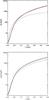 |
Fig. 4 Total magnetic energy amplification as a function of time (a) for different values of the initial magnetic field (upper panel) BIGM = 10-7 μG (solid), BIGM = 10-6 μG (dotted), BIGM = 10-5 μG (dashed) and BIGM = 10-4 μG (dash-dotted), and (b) for different values of the Lagrangian refinement criterion with BIGM = 10-7 μG (bottom panel): mres = m0 is the reference run (solid line), mres = 5 × m0 (dotted line), mres = 25 × m0 (dashed line) and mres = 100 × m0 (dash-dotted line). In each plot, the simple Ω amplification model is overplotted in red for ΩG = 19 Gyr-1 as average angular velocity. |
An important issue is that we attempt to model a quiescent star-forming galaxy with an EoS mimicking the multiphase nature of the ISM gas, i.e. the gas pressure is artificially boosted to take into account the effect of supernovae heating of the ISM. The direct consequence is that the gas distribution is very smooth in the disc (no small scale clumping can develop), and as a consequence, supernova explosions have a very low impact on the ISM. A next step would be to simulate the evolution of a starburst galaxy, within which large clumps (~100 pc size) would be resolved and within which we could hope that supernovae are able to produce a small-scale dynamo effect. In order to get a global dynamo effect, additional physics would also be needed: non-ideal effects like Ohmic or turbulent dissipation and cosmic rays have already been identified as key ingredients to get a strong dynamo (see Hanasz et al. 2009a, for instance).
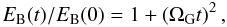
An investigation of the magnetic energy growth within the disc reveals that there is no substantial increase of the magnetic field when SN explosions are allowed in the galaxy (Fig. 5). There are three effects: first, due to supernovae heating (both turbulent and thermal), the early magnetic field amplification appears weaker than in the no-SN case. As a result, the magnetic energy is slightly lower than without SNII. Second, the longer term magnetic field amplification appears slightly more efficient with SN. Finally, the large-scale galactic wind carries some of the magnetic energy available in the disc, producing a slight decrease compared to the simulation without feedback. As a result, the final magnetic energy value is almost equal to the final energy without SN explosions. This is a very weak and subtle effect. We notice that we reproduce almost the same energy evolutions (kinetic, thermal and magnetic) as Wang & Abel (2009). Interestingly, both kinetic and internal energies are lower when feedback proceeds: this is partly due to the gas consumption by the star-forming process, and partly to the ejection of some material from outside the galaxy.
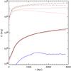 |
Fig. 5 Evolution of the magnetic energy (solid), thermal energy (dotted), and kinetic energy (dashed) for the simulation without star-formation (black) and with SN feedback (red). The initial magnetic field is in both cases BIGM = 10-5 μG, and the energies are computed in a small cube of 15 kpc size around the galaxy. The blue solid line is the magnetic energy for the magnetic seeding simulation (see Appendix). |
The evolution of the magnetic field is rapidly dominated by its tangential component, which
is defined by the cylindrical coordinates (r, θ and
z, where z is the spin axis of the galactic disc). Thus
 (13)when compared to the
evolution of Bθ, which rigorously writes
(13)when compared to the
evolution of Bθ, which rigorously writes
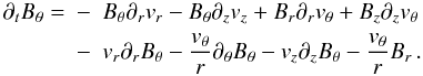 (14)For
an axisymmetric field the amplification is done by the shearing terms, i.e. combining the
third and last terms of this equation, it leads to
(14)For
an axisymmetric field the amplification is done by the shearing terms, i.e. combining the
third and last terms of this equation, it leads to  (15)where we introduce the
angular velocity Ω(r). Then the radial shear governs the evolution of the
magnetic field. We verified that the vertical shear component
(rBz∂zΩ)
is negligible here. If the right-hand side terms of Eq. (15) are not time-dependent, this equation resumes to
(15)where we introduce the
angular velocity Ω(r). Then the radial shear governs the evolution of the
magnetic field. We verified that the vertical shear component
(rBz∂zΩ)
is negligible here. If the right-hand side terms of Eq. (15) are not time-dependent, this equation resumes to  (16)If we assume that
initially the magnetic field is dominated by the radial component, we can derive a very
simple expression for the evolution of the total magnetic energy in the disc by integrating
(16)If we assume that
initially the magnetic field is dominated by the radial component, we can derive a very
simple expression for the evolution of the total magnetic energy in the disc by integrating

 (17)where
 is the average
(
is the average
( weighted) angular velocity squared
of the galaxy. This simple analytical formula compares very well with the actual magnetic
energy amplification we measured in our simulations, as can be seen in Fig. 4. Then one can infer that most of the energy comes from
winding up the radial field within the disk. The best fit to our pure Ω amplification model
on the magnetic energy evolution (Eq. (17))
from our simulations gives ΩG ≃ 19 Gyr-1, which corresponds, using a
simple dimensional analysis, to a disc magnetic scale length
rd ≃ 1.9 kpc for a circular velocity of
V200 = 35 km s-1 (with
ΩG ≃ V200/rd).
This value is consistent with the angular velocity profiles measured at different times
during the course of the simulation (see Fig. 6). Only
in our high magnetic field case,
BIGM = 10-4 μG, do we see a
significant deviation from this simple model. This is due to magnetic braking: angular
momentum is removed from the disc by Alfvén waves propagating along the more rigid field
lines (Hennebelle & Fromang 2008). The
angular velocity of the disc is therefore slowly decreasing. For all the other cases,
magnetic braking is negligible and the magnetic amplification is very similar to the pure Ω
amplification model.
weighted) angular velocity squared
of the galaxy. This simple analytical formula compares very well with the actual magnetic
energy amplification we measured in our simulations, as can be seen in Fig. 4. Then one can infer that most of the energy comes from
winding up the radial field within the disk. The best fit to our pure Ω amplification model
on the magnetic energy evolution (Eq. (17))
from our simulations gives ΩG ≃ 19 Gyr-1, which corresponds, using a
simple dimensional analysis, to a disc magnetic scale length
rd ≃ 1.9 kpc for a circular velocity of
V200 = 35 km s-1 (with
ΩG ≃ V200/rd).
This value is consistent with the angular velocity profiles measured at different times
during the course of the simulation (see Fig. 6). Only
in our high magnetic field case,
BIGM = 10-4 μG, do we see a
significant deviation from this simple model. This is due to magnetic braking: angular
momentum is removed from the disc by Alfvén waves propagating along the more rigid field
lines (Hennebelle & Fromang 2008). The
angular velocity of the disc is therefore slowly decreasing. For all the other cases,
magnetic braking is negligible and the magnetic amplification is very similar to the pure Ω
amplification model.
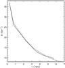 |
Fig. 6 Mass-weighted average angular velocity in the galactic disc as a function of radius at t = 1 Gyr (solid line), t = 2 Gyr (dotted line) and t = 3 Gyr (dashed line) for the simulation without star formation. |
We estimated the effect of mass resolution on the magnetic amplification. Figure 4 shows the measured amplification in four different cases: our fiducial with mres = m0, and three lower mass resolutions with mres = 5, 25 and 100 × m0. The collapsing halo is therefore described with fewer and fewer AMR cells (3 × 10⁶, 8 × 10⁵, 4 × 10⁵ and 3 × 10⁵ total cells in decreasing order of mres). The disc is however always refined at the maximum level of refinement, with a spatial resolution of 150 pc. As a consequence, only our lowest resolution simulation shows a significant deviation from the fiducial case, which can be considered as fully converged within the framework of our sub-grid effective EoS.
A more detailed inspection of the magnetic field amplification shows that the contribution of pure compressional amplification of the magnetic energy (ρ4/3) is dominant in the first 100 Myr of galaxy formation owing to the low-velocity amplitude of the gas in the centre of the NFW profile. But after 200 Myr, this contribution to the magnetic field evolution is negligible compared to the measured magnetic energy in the disc. So it is reasonable to omit considering the amplification by compression over the whole galaxy evolution (which runs over Gyrs).
Our simulation results compare very well with the work presented in Kotarba et al. (2009), where the authors report a similar magnetic amplification using two different SPH codes. They used various force-softening lengths, down to 100 pc, quite similar to our grid spacing. They also used a similar physical model, because they did not allow the gas to cool below 104 K. Although their SPH simulations were all initialised as an initial Milky Way-disc configuration, their results are quite consistent with a pure Ω amplification. In a few cases only did they obtain a faster, exponential growth of magnetic energy. These cases all correspond to numerical schemes where the magnetic divergence was allowed to significantly deviate from zero. They are probably associated with numerical instabilities. In the majority of the SPH results, for which the magnetic divergence was well-behaved, the magnetic energy was growing in the same way as t2.
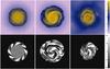 |
Fig. 7 Magnetic amplitude in log μG with magnetic vectors overplotted (upper panels) and the pitch angle θp in degrees (bottom panels) for the galaxy without star formation at t ≃ 3 Gyr (left panels), for the galaxy with star formation and without feedback at t = 4 Gyr (middle panels), and for the galaxy with star formation and supernova feedback at t = 3 Gyr (right panels) in the upper part of the equatorial plan. The initial magnetic field is BIGM = 10-5 μG. The picture size is 40 kpc. |
Wang & Abel (2009), on the other hand, have used an AMR code with a much better spatial resolution (down to 25 pc) and have included cooling processes down to 300 K. In a dwarf galaxy similar to the one studied here, they were able to resolve the fragmentation of gas clumps and the associated vortex modes. But they did not consider star formation and supernova feedback. They concluded that the main amplification mechanism in their simulations was differential rotation: even at the 25 pc resolution they reached, they did not capture any turbulent dynamo and its associated α effect: the magnetic energy was also growing in the same way as t2 in their case.
To support the simple Ω amplification model to explain our simulation results even more, we
now analyse in greater detail the magnetic field morphology in our disc galaxy. We consider
for that purpose three different cases: 1– formation of the disc with only cooling;
2– formation of the disc with cooling and star formation, and finally; 3– formation of the
disc with cooling, star formation, and supernova feedback. The magnetic field morphology is
shown in Fig. 7. We also show in the same figure the
magnetic pitch angle defined as 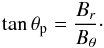 (18)θp
gives the angle between the magnetic field within the horizontal plane and its azimuthal
component. θp = 0° corresponds to pure azimuthal
field lines and θp = 90° to pure radial field lines.
We stress that the pitch angles inferred from observations are obtained with synthetic
polarisation maps from radio emission. Below, we extract a slice of the magnetic field
through the galactic plane to get the pitch angle as defined by Eq. (18), assuming that it provides a good comparison
with observational synthetic polarisation if the pitch is independent of the vertical height
(which is roughly the case in these simulations).
(18)θp
gives the angle between the magnetic field within the horizontal plane and its azimuthal
component. θp = 0° corresponds to pure azimuthal
field lines and θp = 90° to pure radial field lines.
We stress that the pitch angles inferred from observations are obtained with synthetic
polarisation maps from radio emission. Below, we extract a slice of the magnetic field
through the galactic plane to get the pitch angle as defined by Eq. (18), assuming that it provides a good comparison
with observational synthetic polarisation if the pitch is independent of the vertical height
(which is roughly the case in these simulations).
Without any star-formation process, the magnetic field in the galactic disc is almost purely azimuthal: we can see from the left plot in Fig. 7 that the pitch angle then reaches a maximum value of θp = −2°. The gas disc is stabilized by the effective EoS, so that no density perturbation can break the almost perfect azimuthal symmetry (only modes with m = 0 emerge). After the collapse, the radial component of the magnetic field points away from the centre of symmetry above the galactic plane and towards the centre below the plane. Using Eq. (15), we see that the toroidal magnetic field also changes sign above and below the plane: the field is said to be anti-symmetric. This kind of particular symmetry is called the A0 mode (anti-symmetric and m = 0) and emerges naturally in a halo without strong disc-halo interactions (such as galactic winds or galactic fountains) (Beck et al. 1996; Beck 2009). The Milky Way, for example, is believed to be a good example of this A0 magnetic field in the halo (Han et al. 1997; Sun et al. 2008).
The situation appears to be quite different when star formation is taken into account. Because mass is removed from the gas disc to form stars, our effective EoS reaches a lower density and the gas sound speed is lower. The disc Toomre parameter becomes smaller, closer to 1, and a strong spiral mode can develop. We see from the central plot in Fig. 7 that the magnetic field is not axisymmetric anymore. The strong density perturbation triggers fluctuation in the angular velocity, so that Ω(r) is not monotone anymore, but fluctuates around V200/r. We can see again from Eq. (15) that when Br changes sign, the corresponding toroidal component can decrease, or even change sign. We see indeed in Fig. 7 that the toroidal field almost reverts its main direction between the spiral arm and the inter-arm regions. As a consequence, the pitch angle amplitude |θp| is high in the low-density inter-arm regions |θp| ≃ 40° (with both negative and positive signs) and is lower within the spiral arms with |θp| ≃ 20° (always with negative values). These values agree well with the observed pitch angles in nearby galaxies (Beck et al. 1996; Rohde et al. 1999; Patrikeev et al. 2006). The same relation between the pitch angle and the spiral arms is also observed within spiral galaxies: the magnetic field is aligned with the optical spiral arms (Krause et al. 1989; Neininger et al. 1991; Berkhuijsen et al. 1997; Beck 2007), and it also sometimes appears that magnetic fields that are stronger ordered are seen within the inter-arm regions (Ehle et al. 1996; Frick et al. 2000).
Figure 7 clearly shows positive and negative signs of the pitch angle. Therefore a simple spiral density flow cannot explain the observations, which show only negative pitch angles. But spirals may contribute to the increase of the pitch angle compared to a pure axisymmetric rotation, at least at the inner edge of the spirals. Thus, the always negative pitch angle seen in the observations is one of the arguments favouring the dynamo.
The magneto rotational instability (MRI) could also be a growth mode of the magnetic field in galaxies (Kitchatinov & Rüdiger 2004) or sustain turbulence in the disc (Piontek & Ostriker 2005). The MRI can give a coherent picture for the pitch angle of polarised emission if the magnetic field has several reversals along the vertical direction (Elstner et al. 2009). The MRI needs a strong toroïdal field to be efficient, and it is obvious that the field in our galaxy simulations is preferentially poloïdal at late times (see Fig. 7). However, there is a possible MRI channel for the magnetic field growth in the early evolution of the galaxy (<300 Myr) when the circular magnetic component is still lower or comparable to the vertical field then later on the amplification by differential rotation proceeds. But it is beyond the scope of this paper to distinguish this early MRI from the pure differential rotation suggested before and would require simulations with higher resolution to properly describe the MRI-driven turbulence.
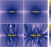 |
Fig. 8 Magnetic field in log μG units for the galaxy with star formation and supernova feedback with BIGM = 10-5 μG at different epochs t = 1 Gyr (upper left), t = 1.5 Gyr (upper right), t = 2 Gyr ( bottom left) and t = 3 Gyr (bottom right). The picture size is 40 kpc. |
When supernova explosions are finally included in the model, the previous magnetic field topology is conserved. The spiral arm is somewhat weaker, because the increased velocity dispersion due to supernova blast waves stabilises the disc. The disc appears less coherent and more perturbed by small scale perturbations. Note that this is precisely the small scale turbulence we need for the α effect, but despite these small scale perturbations, the radial component did not significantly grow in our simulation. The magnetic energy evolution conserves the same properties than in the run without star formation: the differential rotation of the disc is the main driver of the galactic magnetic field in these simulations. We probably need sub-parsec scale resolution in order to resolve supernova-induced cyclonic motions that can drive a turbulent dynamo, like in Balsara et al. (2004). Besides the lack of small scale amplification of the radial component of the field, our simulation recovers most of the qualitative features of galactic dynamo models, which predict a similar pitch-angle distribution and magnetic field topologies (Krasheninnikova et al. 1989; Donner & Brandenburg 1990; Elstner et al. 1992). The existence of this small scale α effect in galaxies was recently shown by direct simulations of Gressel et al. (2008), but the problem of its saturation is still under debate (Brandenburg & Subramanian 2005 for example). The value of the parameter α needs to be rather high in order to obtain a galactic dynamo that is fast enough. The conservation of the total magnetic helicity in the galaxy makes a high value for α very difficult to obtain if there is no exchange of magnetic helicity with the halo. This is why we here prefer to focus on the other consequence of supernova feedback, namely the formation of a strong galactic wind, and how this wind transports the magnetic energy.
6. Magnetic field in the galactic wind
We now study in more detail the properties of the supernova-driven galactic wind, which forms during our simulations. We restrict ourselves to the analysis of the case BIGM = 10-5 μG: we obtained in this case a normal star-forming disc, and in the same time a magnetic field close to equipartition in the gaseous disc. A higher value of BIGM would result in the formation of a non-star-forming torus, while a lower value would give rise to a weakly magnetised galactic disc, significantly below equipartition.
In agreement with the simulations shown in Dubois & Teyssier (2008b), the galactic wind appears at 1.5 Gyr and fully develops during the next Gyr. Figure 8 shows four different snapshots (from 1 to 3 Gyr) of the magnetic field in a plane perpendicular to the disc. These snapshots illustrate the three different phases of the galactic wind, described in more details in Dubois & Teyssier (2008b): 1– the bubbling phase, when the supernova luminosity is too weak to break the ram-pressure of the infalling gas (t = 1 Gyr in Fig. 8); 2– the snow-plow phase, when the supernova luminosity is greater than the ram-pressure of the infalling gas, and the wind starts to propagate through the halo (t = 1.5 Gyr and t = 2 Gyr in Fig. 8); and 3– the blow-away phase, when the wind has reached its final, stationary shape with a characteristic nozzle-like structure (t = 3 Gyr in Fig. 8).
We can see from Fig. 8 that the magnetic field in the wind is highly turbulent, with an average amplitude around 10-3 μG, but showing strong variations within the wind, with highly magnetised filament (as high as 10-1 μG) entrained by low-density bubbles (as low as 10-4 μG). The turbulent structure of the magnetic field is typical of convective flows, with buoyantly rising vortices and their associated shearing motions. The magnetic field lines however appear mainly co-linear to the flow, a magnetic configuration that is actually observed in galaxies with outflows (Brandenburg et al. 1993; Chyży et al. 2006; Heesen et al. 2009). Whether the turbulent flow we observe in the galactic wind amplifies the magnetic field is unclear in our simulation. As we discuss below, the wind magnetic energy is clearly decaying because of the overall expanding flow. Moreover, in the wind region our spatial resolution is slightly degraded (around 300 pc), because the grid has been derefined in this low-density region. This suggests that we are not resolving the small scale magnetic energy amplification due to the turbulent convective flow, which leads to a potential underestimation of the magnetic energy in the wind.
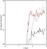 |
Fig. 9 Magnetic energy flux as a function of time for BIGM = 10-5 μG measured at a radius of 4rs (dotted line) and 9rs (dashed line) from the halo centre. The analytical prediction of Bertone et al. (2006) is overplotted as the red solid line. We overploted the result for the direct magnetic energy injection with zero initial magnetic field (solid line) as described in Appendix A. |
In order to estimate the amount of magnetic energy that the wind can extract from the magnetised galactic disc, we measured the magnetic energy flux in two thin shells of a radius 4rs ≃ 20 kpc and 9rs ≃ 45 kpc. Results are shown in Fig. 9. After the wind starts (around t = 1.5 Gyr), the magnetic energy flux quickly jumps to a value of 1052 erg/Gyr, and stays roughly constant during the next Gyr. The magnetic energy flux is decreasing when going to larger radii (roughly as r-1), which demonstrates that the effect of expansion is overcoming the field amplification in the wind turbulence. It seems that the flux still grows after 2 Gyr. It is possible that when the wind reaches a stationary regime, this growth is correlated with the increase of magnetic energy within the disc (see Fig. 5).
It is enlightening to interpret our numerical results in the framework of the analytical
theory of Bertone et al. (2006). This will also guide
our discussion on magnetic field amplification in general. According to Bertone et al. (2006), the magnetic energy flux, which is
injected at the base of the galactic wind, can be written as
 (19)where
Bin is the injected magnetic field,
RG ≃ 7 kpc is the galactic disc radius and
uw is the wind velocity. In their
analytical model, Bertone et al. (2006) first assumed
that the magnetic energy could be considered as some isotropic pressure term. We see from
the previous discussion that the convective turbulence in the wind justifies this
assumption. They also assumed that the injected magnetic field scales with the injected wind
gas density as
(19)where
Bin is the injected magnetic field,
RG ≃ 7 kpc is the galactic disc radius and
uw is the wind velocity. In their
analytical model, Bertone et al. (2006) first assumed
that the magnetic energy could be considered as some isotropic pressure term. We see from
the previous discussion that the convective turbulence in the wind justifies this
assumption. They also assumed that the injected magnetic field scales with the injected wind
gas density as 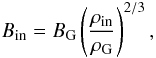 (20)where
BG and ρG are respectively the
typical magnetic field and gas density inside the galactic disc. Finally, they related the
wind gas density to the wind mass flux by
(20)where
BG and ρG are respectively the
typical magnetic field and gas density inside the galactic disc. Finally, they related the
wind gas density to the wind mass flux by
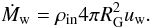 (21)Using the three
previous equations, we can predict the magnetic energy flux in the wind to be
(21)Using the three
previous equations, we can predict the magnetic energy flux in the wind to be 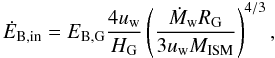 (22)where
HG ≃ 300 pc is the disc thickness and
EB,G is the disc magnetic energy. We
plotted the predicted magnetic energy flux corresponding to Eq. (22) in Fig. 9, using the measured mass flux
(Ṁw ≃ 0.035 M⊙/yr), disc
magnetic energy
(EB,G ≃ 5 × 1053 erg) and disc mass
(MISM ≃ 109 M⊙). We
see that this formula is quite accurate, given the number of simplifying assumptions we
made. It slightly underestimates the measured flux by less than a factor of 2. If we
integrate this magnetic energy flux over tw ≃ 1 Gyr of wind
activity, we find that almost 6% of the disc magnetic energy can be extracted by the
galactic wind and funneled into the IGM. We note with ϵw this
global wind efficiency. In the analytical model of Bertone
et al. (2006), this efficiency writes
(22)where
HG ≃ 300 pc is the disc thickness and
EB,G is the disc magnetic energy. We
plotted the predicted magnetic energy flux corresponding to Eq. (22) in Fig. 9, using the measured mass flux
(Ṁw ≃ 0.035 M⊙/yr), disc
magnetic energy
(EB,G ≃ 5 × 1053 erg) and disc mass
(MISM ≃ 109 M⊙). We
see that this formula is quite accurate, given the number of simplifying assumptions we
made. It slightly underestimates the measured flux by less than a factor of 2. If we
integrate this magnetic energy flux over tw ≃ 1 Gyr of wind
activity, we find that almost 6% of the disc magnetic energy can be extracted by the
galactic wind and funneled into the IGM. We note with ϵw this
global wind efficiency. In the analytical model of Bertone
et al. (2006), this efficiency writes
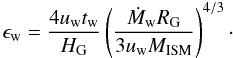 (23)A wind mass injection of
0.03 M⊙/yr is a rather low value compared to starburst
galaxies where these winds are usually observed. Our simulation can be considered as a
quiescent wind case. Typical starburst-driven winds show strong mass outflow as large as
10 M⊙/yr (Martin
1998, 1999). On the other hand, the burst
duration is probably much smaller, with tw ≃ 100 Myr (de Grijs et al. 2001). Overall, the efficiency of the
magnetic energy extraction probably lies above ϵw ≃ 10% for a
typical star-forming dwarf galaxy. The other extreme case one could also consider is when
the starburst is so violent that the whole galaxy is destroyed. This scenario is likely to
happen in the early universe inside small primordial galaxies, as shown by the recent
cosmological simulations of Mashchenko et al. (2008).
The efficiency, then apparently reaches ϵw = 100%.
(23)A wind mass injection of
0.03 M⊙/yr is a rather low value compared to starburst
galaxies where these winds are usually observed. Our simulation can be considered as a
quiescent wind case. Typical starburst-driven winds show strong mass outflow as large as
10 M⊙/yr (Martin
1998, 1999). On the other hand, the burst
duration is probably much smaller, with tw ≃ 100 Myr (de Grijs et al. 2001). Overall, the efficiency of the
magnetic energy extraction probably lies above ϵw ≃ 10% for a
typical star-forming dwarf galaxy. The other extreme case one could also consider is when
the starburst is so violent that the whole galaxy is destroyed. This scenario is likely to
happen in the early universe inside small primordial galaxies, as shown by the recent
cosmological simulations of Mashchenko et al. (2008).
The efficiency, then apparently reaches ϵw = 100%.
We now estimate the magnetic field in the IGM that will result from the enrichment of the
galactic wind. For this purpose, we use the analytical model developed by Bertone et al. (2006) and used recently in a cosmological
simulation by Donnert et al. (2009). We write for the
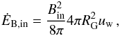
evolution of the magnetic energy in the wind-blown bubble the equation 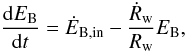 (24)where
ĖB,in is the magnetic energy injection rate,
measured at the base of the expanding wind and Rw is the bubble
radius (with Ṙw its time-derivative). The second term on the
right-hand side of the previous equation stands for magnetic energy losses due to the
expansion of the bubble. This equation also assumes that we can neglect the turbulent
amplification of the magnetic field, which turned out to be true in the simulations we have
performed here. Following Donnert et al. (2009), we
consider the pessimistic case of a fast bubble expansion and write
Ṙw/Rw = 1/t.
We also consider the solution of Eq. (24),
for which the initial bubble energy vanishes
(24)where
ĖB,in is the magnetic energy injection rate,
measured at the base of the expanding wind and Rw is the bubble
radius (with Ṙw its time-derivative). The second term on the
right-hand side of the previous equation stands for magnetic energy losses due to the
expansion of the bubble. This equation also assumes that we can neglect the turbulent
amplification of the magnetic field, which turned out to be true in the simulations we have
performed here. Following Donnert et al. (2009), we
consider the pessimistic case of a fast bubble expansion and write
Ṙw/Rw = 1/t.
We also consider the solution of Eq. (24),
for which the initial bubble energy vanishes
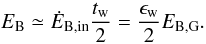 (25)We note that in this
scenario half of the injected energy has been lost owing to the expansion of the field
lines. Using the cosmological wind model of Bertone et al.
(2006), we consider a final wind radius of Rw = 800 kpc
and a wind filling factor of fw = 100% (both typical values for
the universe at redshift zero), so that the final magnetic field in the IGM writes
(25)We note that in this
scenario half of the injected energy has been lost owing to the expansion of the field
lines. Using the cosmological wind model of Bertone et al.
(2006), we consider a final wind radius of Rw = 800 kpc
and a wind filling factor of fw = 100% (both typical values for
the universe at redshift zero), so that the final magnetic field in the IGM writes
 (26)In conclusion, the galactic
wind has enriched the IGM with a magnetic field more than one order of magnitude
larger than its initial value. Interestingly enough, the wind-bubble magnetic
field is proportional to the disc magnetic field. Indeed, the disc magnetic energy depends
on the toroidal magnetic field in the disc as follows
(26)In conclusion, the galactic
wind has enriched the IGM with a magnetic field more than one order of magnitude
larger than its initial value. Interestingly enough, the wind-bubble magnetic
field is proportional to the disc magnetic field. Indeed, the disc magnetic energy depends
on the toroidal magnetic field in the disc as follows
 (27)so that the new IGM
value now writes
(27)so that the new IGM
value now writes  (28)This last formula stands as
a nice and concise summary of our work: we have shown with detailed MHD simulations that the
final magnetic field in the expanding wind bubble inherits its value from the parent dwarf
galaxy, where an Ω effect has amplified the field by almost two orders of magnitude from its
initial value.
(28)This last formula stands as
a nice and concise summary of our work: we have shown with detailed MHD simulations that the
final magnetic field in the expanding wind bubble inherits its value from the parent dwarf
galaxy, where an Ω effect has amplified the field by almost two orders of magnitude from its
initial value.
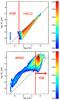 |
Fig. 10 Magnetic amplitude versus gas overdensity diagram at t = 0 Gyr (upper panel) and t = 3 Gyr (bottom pannel) for the galaxy with star formation, supernova feedback and BIGM = 10-5 μG. The black solid line is for the initial ρ2/3 law and the black dashed line is for the initial ρ2/3 law amplified by a factor 60. |
7. Discussion
Using an idealised set-up to model the dwarf galaxy formation with MHD, we followed the
evolution of the magnetic field from the collapse of an equilibrium halo to the formation of
a galactic disc and finally to the ejection of magnetic field lines by a supernova-driven
galactic wind. To illustrate further the mechanism that powers this cosmic cycle in greater
details, for which dwarf galaxies play the central role, we have in Fig. 10 the magnetic phase space diagram, showing a
mass-weighted histogram as a function of the magnetic field amplitude and gas overdensity.
First, when the halo forms, the magnetic field is amplified by gravitational contraction
from its initial IGM value to its final disc value
 (29)We use only the radial
component Br here, because just after collapse
the magnetic field is essentially radial in the disc (see discussion above and Fig. 1). We can see in the upper part of Fig. 10 our initial configuration, where B and
ρ follow this tight relation. Note here that we neglected the additional
amplification of the magnetic field due to turbulent motions in the halo. If we note with
R the initial Lagrangian radius of the collapsing halo and
λ its spin parameter, we know from the standard cosmological
disc-formation model of Mo et al. (1998) that the
final disc radius writes
(29)We use only the radial
component Br here, because just after collapse
the magnetic field is essentially radial in the disc (see discussion above and Fig. 1). We can see in the upper part of Fig. 10 our initial configuration, where B and
ρ follow this tight relation. Note here that we neglected the additional
amplification of the magnetic field due to turbulent motions in the halo. If we note with
R the initial Lagrangian radius of the collapsing halo and
λ its spin parameter, we know from the standard cosmological
disc-formation model of Mo et al. (1998) that the
final disc radius writes  (30)so that the initial disc
radial component writes
(30)so that the initial disc
radial component writes  (31)In the lower panel
of Fig. 10, we see that the toroidal field in the disc
has grown linearly with time due to differential rotation (the Ω amplification) by a factor
of 60, corresponding to the growth rate (Eq. (16)) integrated over 3 Gyr. We finally get the growth rate of the toroidal
magnetic field in the disc as a function of the initial magnetic field in the IGM as
(31)In the lower panel
of Fig. 10, we see that the toroidal field in the disc
has grown linearly with time due to differential rotation (the Ω amplification) by a factor
of 60, corresponding to the growth rate (Eq. (16)) integrated over 3 Gyr. We finally get the growth rate of the toroidal
magnetic field in the disc as a function of the initial magnetic field in the IGM as
 (32)In the lower panel of
Fig. 10 we see that this amplified magnetic field is
funnelled out of the galactic disc, following a
ρ2/3 relation back to the IGM. This is the
“galactic wind” branch that ends the overall cycle. We have seen that the IGM magnetic field
has been amplified by one order of magnitude during this cycle of 3 Gyr.
(32)In the lower panel of
Fig. 10 we see that this amplified magnetic field is
funnelled out of the galactic disc, following a
ρ2/3 relation back to the IGM. This is the
“galactic wind” branch that ends the overall cycle. We have seen that the IGM magnetic field
has been amplified by one order of magnitude during this cycle of 3 Gyr.
Although our simulations, in conjunction with the work presented in Bertone et al. (2006) and Donnert et al. (2009), provide a sufficient explanation for the origin of an IGM magnetic field, at a level as high as 10-4 μG, assuming equipartition magnetic fields in dwarf galaxies, we still need to explain the origin of these intense galactic fields, given that we start our cosmic evolution with a very low initial value BIGM ≃ 10-14 μG immediately after reionisation. We cannot rely on the Ω amplification alone, because there the magnetic field grows only linearly with time. In the context of isolated galaxies, the only source of additional amplification comes from small scale turbulent and cyclonic motions (the α effect). This turbulent dynamo is believed to amplify the radial component of the galactic field, where the toroidal component is generated and amplified by the Ω effect.
We know however that galaxies are far from isolated. They form by accretion of diffuse IGM gas, usually in the form of dense, cold filaments known as cold streams (Dekel et al. 2009), but also by accretion of satellite galaxies, which orbit around the central galaxy before they are incorporated more or less violently into the final disc. These two important processes define the hierarchical scenario of galaxy formation (Silk & White 1978; White & Rees 1978), and probably explain most of the properties of present day galaxies (Governato et al. 2007; Mayer et al. 2008).
We propose here to look at the galactic dynamo problem from a different angle. Instead of relying only on the small scale dynamo to amplify the radial component of the field, we should consider also as a source of radial field:
-
1-
the toroidal magnetic field coming from accreted satellitegalaxies and;
-
2-
the accreted IGM magnetic field previously enriched by galactic winds or;
-
3-
the accreted IGM magnetic field previously enriched by entirely destroyed progenitor galaxies.
On one hand, we know from Eq. (28) that the enriched magnetic field is proportional to the toroidal field of the parent galaxy, and on the other hand, we know from Eq. (32) that the growth rate of the toroidal field of the main galaxy is proportional to the initial IGM magnetic field.
Although a correct description of satellites and cold stream accretion requires detailed
cosmological simulations of galaxy formation with MHD, we can speculate here that our
proposed cycle of accretion and ejection of magnetic field lines (see Fig. 10) probably provides a dynamo loop, for which the radial
field component is amplified by accretion of satellite galaxies and of the magnetically
enriched IGM. A very rough and speculative analytical description of this effect can be
obtained by injecting Eq. (32) into
Eq. (28), 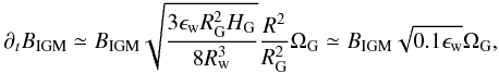 (33)where we exploited the
result of Bertone et al. (2005) that
Rw ≃ 3R (a reasonably good approximation
according to their Fig. 2), and we assumed a typical disc-aspect ratio of
HG/RG ≃ 1/20
and a typical spin parameter λ ≃ 0.05. We see from the previous equation
that now the magnetic field amplification is exponential and not anymore linear, because we
have connected the radial component to the progenitor galaxies’ toroidal component. Although
we have clearly not demonstrated that this cosmic dynamo actually works, we stress that the
cosmological environment provide an important role, namely by accretion of amplified field
lines from diffuse gas or satellite galaxies. The central engines of this cosmic dynamo are
the dwarf galaxies, because they are easily disrupted by galactic winds, and therefore
provide an important source of a diffuse radial field, and also because they are the
progenitors of our Milky Way Galaxy.
(33)where we exploited the
result of Bertone et al. (2005) that
Rw ≃ 3R (a reasonably good approximation
according to their Fig. 2), and we assumed a typical disc-aspect ratio of
HG/RG ≃ 1/20
and a typical spin parameter λ ≃ 0.05. We see from the previous equation
that now the magnetic field amplification is exponential and not anymore linear, because we
have connected the radial component to the progenitor galaxies’ toroidal component. Although
we have clearly not demonstrated that this cosmic dynamo actually works, we stress that the
cosmological environment provide an important role, namely by accretion of amplified field
lines from diffuse gas or satellite galaxies. The central engines of this cosmic dynamo are
the dwarf galaxies, because they are easily disrupted by galactic winds, and therefore
provide an important source of a diffuse radial field, and also because they are the
progenitors of our Milky Way Galaxy.
Some caveats to this cosmic dynamo scenario must be pointed out. We assumed that
BIGM is regenerated in a pure radial mode to get that
exponential growth. Even though magnetic field lines in large-scale bipolar outflows are
mainly perpendicular to the disc (see Heesen et al.
2009, for example), they carry a turbulence that produces non-radial components of
the field. The propagation of the outflow can be affected by the particular geometry of the
galactic environment and leads to irregular distributions of the magnetic field components.
Moreover magnetic fields can contribute constructively or destructively to the
BIGM when large-scale bubbles percolate and can substantially
alter the final configuration of the field. A very rough way of taking these effects on the
radial component into account is to consider that each component of the field is equally
distributed; then Eq. (33) is simply
affected by a factor  .
.
While the α-Ω dynamo comes from the connection between small scale turbulence and galactic differential rotation, the proposed cosmic dynamo originates from the coupling of a large scale gas cycle (cosmological accretion and wind ejection) and differential rotation. We see from Eq. (33) that this effect is probably very fast, especially at high redshift, for which the angular velocity of dwarf galaxies is much higher than today (ΩG ∝ (1 + z)3/2). The actual growth rate will however depend crucially on many complicated aspects of galaxy formation that are beyond the scope of this paper, such as the wind filling factor as a function of redshift (Bertone et al. 2005), the field geometry during satellite mergers, the exact three-dimensional propagation of wind bubbles within the cosmic web, etc. Here it is a priori assumed that the galactic wind expansion in conjunction with some mergers happens within the 3 Gyr. Thus it has to be shown that a similar growth could be achieved with an initial field configuration that is similar to the evolved wind field.
We believe that this cosmic dynamo, in conjunction with a strong galactic dynamo should be able to account for the fast magnetic field amplification we see in our Universe, especially in light of the recent measurements performed on high-redshift galaxies up to redshift 1 (Bernet et al. 2008). Because the existence of an efficient α-Ω Dynamo is questionable in dwarf galaxies owing to the low rotation of the disc and the lack of relativistic particles (Klein 1991), it is important to explore alternative scenarios. It is possible to rely on the ideas discussed by Rees (1987), where stars are able to generate their own magnetic field by stellar dynamos. We tested this scenario in the appendix, showing that for reasonable assumptions we can reach magnetic fields close to equipartition in a few Gyr.
We also demonstrated with our cooling halo simulations that if the IGM magnetic field is high enough (namely BIGM ≃ 10-4 μG), the Lorentz force can prevent the formation of a new generation of dwarf galaxies. The formation of a magnetically supported torus prevents any subsequent star formation, and therefore breaks the central engine of our cosmic dynamo. This has the interesting consequence of providing a saturation mechanism, explaining naturally why the cosmic dynamo leads to a final value of BIGM ≃ 10-5 to 10-4 μG. While the α-Ω dynamo saturates when the small scale turbulent magnetic field reaches equipartition in the disc and magnetic tension becomes able to suppress the small scale dynamo (see Subramanian 1998, Brandenburg & Subramanian 2005), the cosmic dynamo saturates when the large scale cosmological magnetic field prevents dwarf galaxies’ disc formation, or severely affects star formation within them.
The evolution of magnetic fields in galaxies can now be addressed in a cosmological context. In a more or less near future we propose to extend the present work using much higher resolution simulations, the ultimate goal being to resolve the small scale α effect in our isolated, cooling halo simulations. Another ambitious objective would be to address the same problem in a fully cosmological environment, capturing the α effect with some subgrid model, but accounting properly for satellite accretion and wind-bubble propagation.
Acknowledgments
The authors thank Rainer Beck, Katia Ferrière, Sébastien Fromang and Ana Palacios for useful discussions and their valuable comments. This work has been supported by the Horizon Project. Computations were done at CCRT, the CEA Supercomputing Centre.
References
- Alecian, E., Wade, G. A., Catala, C., et al. 2008, A&A, 481, L99 [NASA ADS] [CrossRef] [EDP Sciences] [Google Scholar]
- Arshakian, T. G., Beck, R., Krause, M., & Sokoloff, D. 2009, A&A, 494, 21 [NASA ADS] [CrossRef] [EDP Sciences] [Google Scholar]
- Asai, N., Fukuda, N., & Matsumoto, R. 2007, ApJ, 663, 816 [NASA ADS] [CrossRef] [Google Scholar]
- Balsara, D. S., Kim, J., Mac Low, M.-M., & Mathews, G. J. 2004, ApJ, 617, 339 [NASA ADS] [CrossRef] [Google Scholar]
- Bate, M. R., & Burkert, A. 1997, MNRAS, 288, 1060 [NASA ADS] [CrossRef] [Google Scholar]
- Beck, R. 2007, A&A, 470, 539 [NASA ADS] [CrossRef] [EDP Sciences] [Google Scholar]
- Beck, R. 2009, Ap&SS, 320, 77 [NASA ADS] [CrossRef] [Google Scholar]
- Beck, R., Brandenburg, A., Moss, D., Shukurov, A., & Sokoloff, D. 1996, ARA&A, 34, 155 [NASA ADS] [CrossRef] [Google Scholar]
- Bell, A. R. 2004, MNRAS, 353, 550 [Google Scholar]
- Berkhuijsen, E. M., Horellou, C., Krause, M., et al. 1997, A&A, 318, 700 [NASA ADS] [Google Scholar]
- Bernet, M. L., Miniati, F., Lilly, S. J., Kronberg, P. P., & Dessauges-Zavadsky, M. 2008, Nature, 454, 302 [NASA ADS] [CrossRef] [PubMed] [Google Scholar]
- Bertone, S., Stoehr, F., & White, S. D. M. 2005, MNRAS, 359, 1201 [NASA ADS] [CrossRef] [Google Scholar]
- Bertone, S., Vogt, C., & Enßlin, T. 2006, MNRAS, 370, 319 [NASA ADS] [Google Scholar]
- Blasi, P., Burles, S., & Olinto, A. V. 1999, ApJ, 514, L79 [NASA ADS] [CrossRef] [Google Scholar]
- Brandenburg, A., & Subramanian, K. 2005, Phys. Rep., 417, 1 [NASA ADS] [CrossRef] [Google Scholar]
- Brandenburg, A., Donner, K. J., Moss, D., et al. 1993, A&A, 271, 36 [NASA ADS] [Google Scholar]
- Brandenburg, A., Nordlund, A., Stein, R. F., & Torkelsson, U. 1995, ApJ, 446, 741 [NASA ADS] [CrossRef] [Google Scholar]
- Brüggen, M., Ruszkowski, M., Simionescu, A., Hoeft, M., & Dalla Vecchia, C. 2005, ApJ, 631, L21 [NASA ADS] [CrossRef] [Google Scholar]
- Brun, A. S., Miesch, M. S., & Toomre, J. 2004, ApJ, 614, 1073 [NASA ADS] [CrossRef] [Google Scholar]
- Bullock, J. S., Dekel, A., Kolatt, T. S., et al. 2001, ApJ, 555, 240 [NASA ADS] [CrossRef] [Google Scholar]
- Carilli, C. L., & Taylor, G. B. 2002, ARA&A, 40, 319 [NASA ADS] [CrossRef] [Google Scholar]
- Cattaneo, F., & Hughes, D. W. 1996, Phys. Rev. E, 54, 4532 [NASA ADS] [CrossRef] [Google Scholar]
- Ceverino, D., & Klypin, A. 2009, ApJ, 695, 292 [NASA ADS] [CrossRef] [Google Scholar]
- Charbonneau, P., & MacGregor, K. B. 2001, ApJ, 559, 1094 [Google Scholar]
- Cheng, B., Schramm, D. N., & Truran, J. W. 1994, Phys. Rev. D, 49, 5006 [NASA ADS] [CrossRef] [Google Scholar]
- Chyży, K. T., Soida, M., Bomans, D. J., et al. 2006, A&A, 447, 465 [NASA ADS] [CrossRef] [EDP Sciences] [Google Scholar]
- Dal la Vecchia, C., & Schaye, J. 2008, MNRAS, 387, 1431 [NASA ADS] [CrossRef] [Google Scholar]
- de Grijs, R., O’Connell, R. W., & Gallagher III, J. S. 2001, AJ, 121, 768 [NASA ADS] [CrossRef] [Google Scholar]
- Dekel, A., Birnboim, Y., Engel, G., et al. 2009, Nature, 457, 451 [NASA ADS] [CrossRef] [PubMed] [Google Scholar]
- Dolag, K., Bartelmann, M., & Lesch, H. 1999, A&A, 348, 351 [NASA ADS] [Google Scholar]
- Dolag, K., Bartelmann, M., & Lesch, H. 2002, A&A, 387, 383 [NASA ADS] [CrossRef] [EDP Sciences] [Google Scholar]
- Dolag, K., Grasso, D., Springel, V., & Tkachev, I. 2005, J. Cosmol. Astro-Part. Phys., 1, 9 [Google Scholar]
- Donner, K. J., & Brandenburg, A. 1990, A&A, 240, 289 [NASA ADS] [Google Scholar]
- Donnert, J., Dolag, K., Lesch, H., & Müller, E. 2009, MNRAS, 392, 1008 [NASA ADS] [CrossRef] [Google Scholar]
- Dubois, Y., & Teyssier, R. 2008a, A&A, 482, L13 [NASA ADS] [CrossRef] [EDP Sciences] [Google Scholar]
- Dubois, Y., & Teyssier, R. 2008b, A&A, 477, 79 [NASA ADS] [CrossRef] [EDP Sciences] [Google Scholar]
- Dubois, Y., Devriendt, J., Slyz, A., & Silk, J. 2009, MNRAS, 399, L49 [NASA ADS] [Google Scholar]
- Efstathiou, G. 2000, MNRAS, 317, 697 [NASA ADS] [CrossRef] [Google Scholar]
- Ehle, M., Beck, R., Haynes, R. F., et al. 1996, A&A, 306, 73 [NASA ADS] [Google Scholar]
- Elstner, D., Meinel, R., & Beck, R. 1992, A&AS, 94, 587 [Google Scholar]
- Elstner, D., Gressel, O., & Rüdiger, G. 2009, in IAU Symp., 259, 467 [NASA ADS] [Google Scholar]
- Enqvist, K., Semikoz, V., Shukurov, A., & Sokoloff, D. 1993, Phys. Rev. D, 48, 4557 [NASA ADS] [CrossRef] [Google Scholar]
- Ferriere, K. 1992a, ApJ, 389, 286 [NASA ADS] [CrossRef] [Google Scholar]
- Ferriere, K. 1992b, ApJ, 391, 188 [NASA ADS] [CrossRef] [Google Scholar]
- Ferrière, K., & Schmitt, D. 2000, A&A, 358, 125 [NASA ADS] [Google Scholar]
- Field, G. B. 1995, in The Physics of the Interstellar Medium and Intergalactic Medium, ed. A. Ferrara, C. F. McKee, C. Heiles, & P. R. Shapiro, ASP, Conf. Ser., 80, 1 [Google Scholar]
- Frick, P., Beck, R., Shukurov, A., et al. 2000, MNRAS, 318, 925 [NASA ADS] [CrossRef] [Google Scholar]
- Fromang, S., Hennebelle, P., & Teyssier, R. 2006, A&A, 457, 371 [NASA ADS] [CrossRef] [EDP Sciences] [Google Scholar]
- Gissinger, C., Fromang, S., & Dormy, E. 2009, MNRAS, 394, L84 [NASA ADS] [Google Scholar]
- Gnedin, N. Y., Ferrara, A., & Zweibel, E. G. 2000, ApJ, 539, 505 [NASA ADS] [CrossRef] [Google Scholar]
- Governato, F., Willman, B., Mayer, L., et al. 2007, MNRAS, 374, 1479 [NASA ADS] [CrossRef] [Google Scholar]
- Govoni, F., & Feretti, L. 2004, Intern. J. Mod. Phys. D., 13, 1549 [NASA ADS] [CrossRef] [Google Scholar]
- Grasso, D., & Rubinstein, H. R. 2001, Phys. Rep., 348, 163 [NASA ADS] [CrossRef] [Google Scholar]
- Gressel, O., Elstner, D., Ziegler, U., & Rüdiger, G. 2008, A&A, 486, L35 [NASA ADS] [CrossRef] [EDP Sciences] [Google Scholar]
- Han, J. L., Manchester, R. N., Berkhuijsen, E. M., & Beck, R. 1997, A&A, 322, 98 [NASA ADS] [Google Scholar]
- Hanasz, M., Kowal, G., Otmianowska-Mazur, K., & Lesch, H. 2004, ApJ, 605, L33 [NASA ADS] [CrossRef] [Google Scholar]
- Hanasz, M., Otmianowska-Mazur, K., Kowal, G., & Lesch, H. 2009a, A&A, 498, 335 [NASA ADS] [CrossRef] [EDP Sciences] [Google Scholar]
- Hanasz, M., Wóltański, D., & Kowalik, K. 2009b, ApJ, 706, L155 [NASA ADS] [CrossRef] [Google Scholar]
- Hanayama, H., Takahashi, K., Kotake, K., et al. 2005, ApJ, 633, 941 [NASA ADS] [CrossRef] [Google Scholar]
- Heesen, V., Krause, M., Beck, R., & Dettmar, R. 2009, A&A, 506, 1123 [NASA ADS] [CrossRef] [EDP Sciences] [Google Scholar]
- Helfand, D. J., Gotthelf, E. V., & Halpern, J. P. 2001, ApJ, 556, 380 [NASA ADS] [CrossRef] [Google Scholar]
- Hennebelle, P., & Fromang, S. 2008, A&A, 477, 9 [NASA ADS] [CrossRef] [EDP Sciences] [Google Scholar]
- Hubrig, S., Schöller, M., Schnerr, R. S., et al. 2008, A&A, 490, 793 [NASA ADS] [CrossRef] [EDP Sciences] [Google Scholar]
- Kaufmann, T., Bullock, J. S., Maller, A. H., Fang, T., & Wadsley, J. 2009, MNRAS, 396, 191 [NASA ADS] [CrossRef] [Google Scholar]
- Kennel, C. F., & Coroniti, F. V. 1984, ApJ, 283, 694 [NASA ADS] [CrossRef] [Google Scholar]
- Kitchatinov, L. L., & Rüdiger, G. 2004, A&A, 424, 565 [NASA ADS] [CrossRef] [EDP Sciences] [Google Scholar]
- Klein, U. 1991, Proc. Astron. Soc. Austr., 9, 253 [NASA ADS] [Google Scholar]
- Kotarba, H., Lesch, H., Dolag, K., et al. 2009, MNRAS, 397, 733 [NASA ADS] [CrossRef] [Google Scholar]
- Krasheninnikova, I., Shukurov, A., Ruzmaikin, A., & Sokolov, D. 1989, A&A, 213, 19 [NASA ADS] [Google Scholar]
- Krause, M., Beck, R., & Hummel, E. 1989, A&A, 217, 17 [NASA ADS] [Google Scholar]
- Kronberg, P. P., Lesch, H., & Hopp, U. 1999, ApJ, 511, 56 [NASA ADS] [CrossRef] [Google Scholar]
- Kulsrud, R. M. 1999, ARA&A, 37, 37 [NASA ADS] [CrossRef] [Google Scholar]
- Kroupa, P. 2001, MNRAS, 322, 231 [NASA ADS] [CrossRef] [Google Scholar]
- Kulsrud, R. M., Cen, R., Ostriker, J. P., & Ryu, D. 1997, ApJ, 480, 481 [NASA ADS] [CrossRef] [Google Scholar]
- Kulsrud, R. M., & Zweibel, E. G. 2008, Rep. Prog. Phys., 71, 046901 [NASA ADS] [CrossRef] [Google Scholar]
- MacDonald, J., & Mullan, D. J. 2004, MNRAS, 348, 702 [NASA ADS] [CrossRef] [Google Scholar]
- Machacek, M. E., Bryan, G. L., & Abel, T. 2001, ApJ, 548, 509 [NASA ADS] [CrossRef] [Google Scholar]
- Maeder, A., Georgy, C., & Meynet, G. 2008, A&A, 479, L37 [NASA ADS] [CrossRef] [EDP Sciences] [Google Scholar]
- Martin, C. L. 1998, ApJ, 506, 222 [NASA ADS] [CrossRef] [Google Scholar]
- Martin, C. L. 1999, ApJ, 513, 156 [NASA ADS] [CrossRef] [Google Scholar]
- Mashchenko, S., Wadsley, J., & Couchman, H. M. P. 2008, Science, 319, 174 [NASA ADS] [CrossRef] [Google Scholar]
- Mayer, L., Governato, F., & Kaufmann, T. 2008, Adv. Sci. Lett., 1, 7 [Google Scholar]
- Miyoshi, T., & Kusano, K. 2005, J. Comput. Phys., 208, 315 [NASA ADS] [CrossRef] [Google Scholar]
- Mo, H. J., Mao, S., & White, S. D. M. 1998, MNRAS, 295, 319 [Google Scholar]
- Mullan, D. J., & MacDonald, J. 2005, MNRAS, 356, 1139 [NASA ADS] [CrossRef] [Google Scholar]
- Navarro, J. F., Frenk, C. S., & White, S. D. M. 1996, ApJ, 462, 563 [NASA ADS] [CrossRef] [Google Scholar]
- Neininger, N., Klein, U., Beck, R., & Wielebinski, R. 1991, Nature, 352, 781 [NASA ADS] [CrossRef] [Google Scholar]
- Parker, E. N. 1971, ApJ, 163, 255 [NASA ADS] [CrossRef] [Google Scholar]
- Parker, E. N. 1992, ApJ, 401, 137 [NASA ADS] [CrossRef] [Google Scholar]
- Patrikeev, I., Fletcher, A., Stepanov, R., et al. 2006, A&A, 458, 441 [NASA ADS] [CrossRef] [EDP Sciences] [Google Scholar]
- Piontek, R. A., & Ostriker, E. C. 2005, ApJ, 629, 849 [NASA ADS] [CrossRef] [Google Scholar]
- Rasera, Y., & Teyssier, R. 2006, A&A, 445, 1 [NASA ADS] [CrossRef] [EDP Sciences] [Google Scholar]
- Rees, M. J. 1987, Quart. J. RAS, 28, 197 [Google Scholar]
- Roettiger, K., Stone, J. M., & Burns, J. O. 1999, ApJ, 518, 594 [NASA ADS] [CrossRef] [Google Scholar]
- Rohde, R., Beck, R., & Elstner, D. 1999, A&A, 350, 423 [NASA ADS] [Google Scholar]
- Sciama, D. W. 1994, in Cosmical Magnetism, ed. D. Lynden-Bell, 128–133 [Google Scholar]
- Shukurov, A. 2004, ArXiv Astrophysics e-prints [Google Scholar]
- Sigl, G., Miniati, F., & Enßlin, T. A. 2004, Phys. Rev. D, 70, 043007 [NASA ADS] [CrossRef] [Google Scholar]
- Silk, J., & White, S. D. 1978, ApJ, 223, L59 [NASA ADS] [CrossRef] [Google Scholar]
- Springel, V., & Hernquist, L. 2003, MNRAS, 339, 289 [Google Scholar]
- Subramanian, K. 1998, MNRAS, 294, 718 [NASA ADS] [CrossRef] [Google Scholar]
- Subramanian, K., Shukurov, A., & Haugen, N. E. L. 2006, MNRAS, 366, 1437 [NASA ADS] [CrossRef] [Google Scholar]
- Sun, X. H., Reich, W., Waelkens, A., & Enßlin, T. A. 2008, A&A, 477, 573 [NASA ADS] [CrossRef] [EDP Sciences] [Google Scholar]
- Sutherland, R. S., & Dopita, M. A. 1993, ApJS, 88, 253 [NASA ADS] [CrossRef] [Google Scholar]
- Teyssier, R. 2002, A&A, 385, 337 [NASA ADS] [CrossRef] [EDP Sciences] [Google Scholar]
- Teyssier, R., Fromang, S., & Dormy, E. 2006, J. Comput. Phys., 218, 44 [NASA ADS] [CrossRef] [Google Scholar]
- Truelove, J. K., Klein, R. I., McKee, C. F., et al. 1997, ApJ, 489, L179 [NASA ADS] [CrossRef] [Google Scholar]
- Turner, M. S., & Widrow, L. M. 1988, Phys. Rev. D, 37, 2743 [NASA ADS] [CrossRef] [Google Scholar]
- Wang, P., & Abel, T. 2009, ApJ, 696, 96 [NASA ADS] [CrossRef] [Google Scholar]
- White, S. D. M., & Rees, M. J. 1978, MNRAS, 183, 341 [NASA ADS] [CrossRef] [Google Scholar]
- Wielebinski, R., & Krause, F. 1993, A&A Rev., 4, 449 [Google Scholar]
- Xu, H., O’Shea, B. W., Collins, D. C., et al. 2008, ApJ, 688, L57 [NASA ADS] [CrossRef] [Google Scholar]
- Yepes, G., Kates, R., Khokhlov, A., & Klypin, A. 1997, MNRAS, 284, 235 [NASA ADS] [CrossRef] [Google Scholar]
- Zahn, J.-P., Brun, A. S., & Mathis, S. 2007, A&A, 474, 145 [NASA ADS] [CrossRef] [EDP Sciences] [Google Scholar]
Appendix A: Stellar magnetic feedback scenario
Rees (1987) was the first to suggest that Biermann battery effects at the surface of stars could create magnetic fields from a zero field. We also know that convective stars can amplify the magnetic energy extremely fast (Brun et al. 2004) close to its equipartition value by dynamo effects like in the Sun. In this scenario, massive stars >10 M⊙, which will release their magnetic energy into the ISM in powerful explosions, are the key ingredient for generating galactic magnetic fields. In the most massive stars, it seems that there is no convective envelope allowing for a very fast dynamo, but differential rotation could be extremely strong (Maeder et al. 2008) and can substantially increase any seed field. In some massive stars the convective zone can be in the central part (Zahn et al. 2007) and the dynamo can be effective (Charbonneau & MacGregor 2001). These stars also have a very short life-time (a few Myr), any amplification process must have an extremely short e-folding time. Some models predict that instabilities in the external radiative envelope are able to sustain a sufficiently fast growth of the field (MacDonald & Mullan 2004; Mullan & MacDonald 2005). Though it remains difficult to conclude whether the magnetic field is appreciably amplified, there is increasing observational evidence for strong magnetic fields in massive stars (Alecian et al. 2008; Hubrig et al. 2008).
When a supernova explodes, its magnetic field is diluted in a larger volume. We can
approximate its final value by considering the flux conservation of the magnetic field.
The uniform and averaged magnetic field in a spherical transformation must follow
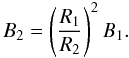 (A.1)For example the Crab
nebula with B1 ≃ 100 μG within a
R1 ≃ 3.4 pc radius (Kennel
& Coroniti 1984) will have a
B2 = 5 × 10⁻² μG field within
the radius R2 = 150 pc of a superbubble. The Crab nebula is a
very strong particular case: a fast rotating pulsar inside the centre of the remnant could
be responsible for this very high magnetic field. It is particularly difficult to explain
how strong magnetic fields
B1 ~ 109 μG in massive stars
(Alecian et al. 2008,
R1 ~ 5 R⊙ ~ 3 × 10⁶ km)
can produce these high values in supernova remants
(B2 ~ 10-5 μG for
R2 ~ 1 pc). This prediction does not take into account the
possible amplification stages during the rapid expansion of the blast wave, the magnetic
field can grow due to the cosmic ray pressure (Parker
1992), some strong Biermann battery effect (Hanayama et al. 2005), or turbulence (Bell
2004), which would allow for higher values in supernova remnants.
(A.1)For example the Crab
nebula with B1 ≃ 100 μG within a
R1 ≃ 3.4 pc radius (Kennel
& Coroniti 1984) will have a
B2 = 5 × 10⁻² μG field within
the radius R2 = 150 pc of a superbubble. The Crab nebula is a
very strong particular case: a fast rotating pulsar inside the centre of the remnant could
be responsible for this very high magnetic field. It is particularly difficult to explain
how strong magnetic fields
B1 ~ 109 μG in massive stars
(Alecian et al. 2008,
R1 ~ 5 R⊙ ~ 3 × 10⁶ km)
can produce these high values in supernova remants
(B2 ~ 10-5 μG for
R2 ~ 1 pc). This prediction does not take into account the
possible amplification stages during the rapid expansion of the blast wave, the magnetic
field can grow due to the cosmic ray pressure (Parker
1992), some strong Biermann battery effect (Hanayama et al. 2005), or turbulence (Bell
2004), which would allow for higher values in supernova remnants.
The basic idea to implement the release of magnetic field by superbubbles coming from supernova explosions is to put a fixed total magnetic energy within the bubble (ensuring that ∇.B = 0) with a random direction. We assume that within a rbubble ≃ 150 pc radius, each supernova constructively contributes for a certain amount of magnetic energy to the final release. We arbitrary choose that each superbubble (which corresponds to an assembly of several individual supernova explosions) releases a 10-3 μG field following a robust numerical implementation. This particular choice of 10-3 μG magnetic seeding is entirely heuristic and is set to match μG field after 1 Gyr of galactic evolution. To get a rough idea of the magnetic release by a single supernova inflating a larger bubble, we have to know the number of supernovae per star cluster particle NSN, ∗ = m∗ × ηSN/MSN ≃ 100, where we have assumed that MSN = 10 M⊙ and for m∗ = n0 × Δx3 ≃ 104 M⊙. To simplify if we assume that each single supernova produces a magnetic field with the exact same intensity and direction, we obtain that the associated magnetic field per supernova (10 M⊙) is BSN ≃ 10-5 μG (in a 150 pc radius bubble). We do not take into account the destructive contributions (magnetic field in opposite directions) but neither do we take into account the substantial increase coming from shocks between supernova explosions that generate instabilities, shear flows, cosmic rays, etc.
 |
Fig. A.1 Magnetic amplitude for the (A.3) dipolar distribution where m is aligned with the z-axis. The upper panel is a slice through the (Oyz) plane and the bottom panel shows a slice through the (Oxy) plane. The magnetic vectors are overplotted. The picture size is 5rSN. |
 |
Fig. A.2 Magnetic amplitude in log μG units with magnetic vectors for the galaxy with star formation, supernova feedback, BIGM = 0, and a magnetic seeding BSN = 10-5 μG at t ≃ 3 Gyr in the (Oyz) plane (upper panel), in the (Oxy) plane (middle panel) and the pitch angle (bottom panel) . The picture size is 40 kpc. |
To implement a method of direct injection of the magnetic energy in the code, we must
find a form of the magnetic field that ensures
∇.B = 0. For that purpose we will design
a dipolar moment configuration in a way that the resulting magnetic field is embedded in
the radius of the supernova explosion, and that the magnetic energy is not divergent in
the centre in order to preserve the stability of the scheme even at different resolutions.
Let us recall that the magnetic potential vector created by a unique magnetic dipole
follows 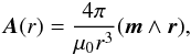 (A.2)where
m is the magnetic dipolar moment. If we
take m as a constant value, one can easily see that
magnetic field will be infinite in the centre, then we must choose a certain distribution
of dipolar moment elements in a way that the overall resulting moment respects the compact
and convergent criteria. For that purpose we need m to grow
as fast as r4, which sharply decreases down to zero at a
certain radius rSN
(A.2)where
m is the magnetic dipolar moment. If we
take m as a constant value, one can easily see that
magnetic field will be infinite in the centre, then we must choose a certain distribution
of dipolar moment elements in a way that the overall resulting moment respects the compact
and convergent criteria. For that purpose we need m to grow
as fast as r4, which sharply decreases down to zero at a
certain radius rSN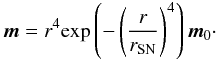 (A.3)With this distribution
of m, we can compute the magnetic field as
(A.3)With this distribution
of m, we can compute the magnetic field as
 (A.4)The resulting
magnetic field computed on a 5123 grid within a
5rSN box size (resolution element is
0.01 rSN) is plotted in Fig. A.1. We can renormalise the dipolar moment distribution so that the
magnetic field gives a unit magnetic energy with regard to the measured magnetic energy
Em, here
(A.4)The resulting
magnetic field computed on a 5123 grid within a
5rSN box size (resolution element is
0.01 rSN) is plotted in Fig. A.1. We can renormalise the dipolar moment distribution so that the
magnetic field gives a unit magnetic energy with regard to the measured magnetic energy
Em, here
 (A.5)This value is
not very sensitive to the numerical resolution, for example, if
Δx = 0.3rSN, then
m0 = 1. That means that even if we poorly resolve the bubble
(which is the case in our simulations
rSN ≃ 2–3Δx), the final magnetic energy is
very close to the converged one.
(A.5)This value is
not very sensitive to the numerical resolution, for example, if
Δx = 0.3rSN, then
m0 = 1. That means that even if we poorly resolve the bubble
(which is the case in our simulations
rSN ≃ 2–3Δx), the final magnetic energy is
very close to the converged one.
We also add a saturation factor to avoid that the magnetic field grows excessively above
the equipartition value, so that the resulting field is multiplied by
 (A.6)where B
is the value of the magnetic field inside the bubble and Beq
is the magnetic amplitude corresponding to its equipartition state with internal energy.
For each buble, the fsat factor is the maximum of all
individual fsat,i factors computed on each
cell within the supernova radius. These saturation effects have been outlined in galactic
dynamo simulations (Cattaneo & Hughes
1996).
(A.6)where B
is the value of the magnetic field inside the bubble and Beq
is the magnetic amplitude corresponding to its equipartition state with internal energy.
For each buble, the fsat factor is the maximum of all
individual fsat,i factors computed on each
cell within the supernova radius. These saturation effects have been outlined in galactic
dynamo simulations (Cattaneo & Hughes
1996).
We produced the exact same simulation as in Sect. 6 with no initial magnetic field. Magnetic fields are randomly generated in the disc, but they tend to align with the global rotation within the disc as one can see in Fig. A.2. After 3 Gyr, the amplitude has reached a value of a few ~10-2 μG in the central parts and its configuration is no longer like a A0 type. Because there is no longer an initial magnetic field, the A0 configuration does not appear. Moreover the randomisation of the magnetic field injection destroys any particular symmetry and reconnects the field through the equatorial plane. This effect explains the smaller scale of the magnetic field fluctuations, but the global differential rotation of the galaxy maintains a preferred component of the field along the rotating vector. A direct consequence of the differential rotation is the amplification applied on magnetic seeds. A computation of the injected magnetic energy from supernovae with the star-formation rate gives Einj ≃ 1048 erg/Gyr. Though the magnetic energy in the disc should reach 1048 erg after 1 Gyr, Fig. 5 shows that the energy measured in the galaxy for this simulation (blue line) is ~3 × 1049 erg after 1 Gyr. This is evidence that the differential rotation still amplifies the seed field generated by supernovae.
Radial contribution is non-negligible, the pitch angle |θp| is everywhere greater than 10° and goes up to 90° in some regions of the galaxy. The 10° minimum value is predictable: if the mean field amplitude is about ~10-2 μG preferentially toroidal, putting a 10-3 μG field in the supernova remnant along the radial component produces a |θp| ≃ 5° pitch angle. Then the successive explosions and the differential rotation make this value rise up to 90°.
As shown in Fig. 9, the magnetic energy flux is lower than when the simulation starts with an initial magnetic field by a factor ~40, but this value depends a lot on the particular choice of the magnetic seeding BSN = 10-5 μG. Thus, with a EB, in ≃ 1051 erg.Gyr-1 at the bottom of the wind, we can predict that the final magnetic field within the hot tenuous bubble will reach ~10-5 μG. This corresponds to the initial cosmological seeds required in large-scale cosmological simulations (Dolag et al. 2005; Dubois & Teyssier 2008a). Relying on the assumption that some supernova remnants (Crab nebula, Vela nebula) are permeated with strong magnetic fields (Kennel & Coroniti 1984; Helfand et al. 2001) we verify that this mechanism can magnetise a dwarf galaxy and therefore produce a magnetised wind to enrich the IGM. Using a very low magnetic seed within supernova bubbles (with a magnetic amplitude that is 5000 times weaker than the field within the Crab nebulae), we showed that the galaxy rapidly reaches 1 μG in ~1 Gyr and is able to fill the IGM with a large-scale magnetic field of ~10-5 μG. It is therefore sufficient to explain an early magnetisation of the Universe.
All Figures
|
Fig. 1 (Oyz) slice of the initial magnetic field amplitude in log μG units and magnetic vectors for BIGM = 10-5 μG at t = 0 Gyr (left pannel) and t = 3 Gyr (right pannel). The picture size is 40 kpc. |
| In the text | |
|
Fig. 2 Magnetic amplitude along the z-axis for different normalisations of the initial profile: BIGM = 10-6 μG (dot-dashed), BIGM = 10-5 μG (dashed) and BIGM = 10-4 μG (dotted). The solid line shows for comparison the magnetic field that would have been in equipartition throughout the halo. |
| In the text | |
|
Fig. 3 Slice through the (Oxz) plane of the gas density in log H/cm-3 (first row), of the temperature in log K (second row), of the magnetic amplitude in log μG (third row), and of the β parameter in log β (fourth row) for an initial magnetic field of BIGM = 10-4 μG (left column), BIGM = 10-5 μG (middle column) and BIGM = 10-6 μG (right column) at t ≃ 3 Gyr. The picture size is 40 kpc. |
| In the text | |
|
Fig. 4 Total magnetic energy amplification as a function of time (a) for different values of the initial magnetic field (upper panel) BIGM = 10-7 μG (solid), BIGM = 10-6 μG (dotted), BIGM = 10-5 μG (dashed) and BIGM = 10-4 μG (dash-dotted), and (b) for different values of the Lagrangian refinement criterion with BIGM = 10-7 μG (bottom panel): mres = m0 is the reference run (solid line), mres = 5 × m0 (dotted line), mres = 25 × m0 (dashed line) and mres = 100 × m0 (dash-dotted line). In each plot, the simple Ω amplification model is overplotted in red for ΩG = 19 Gyr-1 as average angular velocity. |
| In the text | |
|
Fig. 5 Evolution of the magnetic energy (solid), thermal energy (dotted), and kinetic energy (dashed) for the simulation without star-formation (black) and with SN feedback (red). The initial magnetic field is in both cases BIGM = 10-5 μG, and the energies are computed in a small cube of 15 kpc size around the galaxy. The blue solid line is the magnetic energy for the magnetic seeding simulation (see Appendix). |
| In the text | |
|
Fig. 6 Mass-weighted average angular velocity in the galactic disc as a function of radius at t = 1 Gyr (solid line), t = 2 Gyr (dotted line) and t = 3 Gyr (dashed line) for the simulation without star formation. |
| In the text | |
|
Fig. 7 Magnetic amplitude in log μG with magnetic vectors overplotted (upper panels) and the pitch angle θp in degrees (bottom panels) for the galaxy without star formation at t ≃ 3 Gyr (left panels), for the galaxy with star formation and without feedback at t = 4 Gyr (middle panels), and for the galaxy with star formation and supernova feedback at t = 3 Gyr (right panels) in the upper part of the equatorial plan. The initial magnetic field is BIGM = 10-5 μG. The picture size is 40 kpc. |
| In the text | |
|
Fig. 8 Magnetic field in log μG units for the galaxy with star formation and supernova feedback with BIGM = 10-5 μG at different epochs t = 1 Gyr (upper left), t = 1.5 Gyr (upper right), t = 2 Gyr ( bottom left) and t = 3 Gyr (bottom right). The picture size is 40 kpc. |
| In the text | |
|
Fig. 9 Magnetic energy flux as a function of time for BIGM = 10-5 μG measured at a radius of 4rs (dotted line) and 9rs (dashed line) from the halo centre. The analytical prediction of Bertone et al. (2006) is overplotted as the red solid line. We overploted the result for the direct magnetic energy injection with zero initial magnetic field (solid line) as described in Appendix A. |
| In the text | |
|
Fig. 10 Magnetic amplitude versus gas overdensity diagram at t = 0 Gyr (upper panel) and t = 3 Gyr (bottom pannel) for the galaxy with star formation, supernova feedback and BIGM = 10-5 μG. The black solid line is for the initial ρ2/3 law and the black dashed line is for the initial ρ2/3 law amplified by a factor 60. |
| In the text | |
|
Fig. A.1 Magnetic amplitude for the (A.3) dipolar distribution where m is aligned with the z-axis. The upper panel is a slice through the (Oyz) plane and the bottom panel shows a slice through the (Oxy) plane. The magnetic vectors are overplotted. The picture size is 5rSN. |
| In the text | |
|
Fig. A.2 Magnetic amplitude in log μG units with magnetic vectors for the galaxy with star formation, supernova feedback, BIGM = 0, and a magnetic seeding BSN = 10-5 μG at t ≃ 3 Gyr in the (Oyz) plane (upper panel), in the (Oxy) plane (middle panel) and the pitch angle (bottom panel) . The picture size is 40 kpc. |
| In the text | |
Current usage metrics show cumulative count of Article Views (full-text article views including HTML views, PDF and ePub downloads, according to the available data) and Abstracts Views on Vision4Press platform.
Data correspond to usage on the plateform after 2015. The current usage metrics is available 48-96 hours after online publication and is updated daily on week days.
Initial download of the metrics may take a while.