| Issue |
A&A
Volume 513, April 2010
|
|
|---|---|---|
| Article Number | A5 | |
| Number of page(s) | 22 | |
| Section | Interstellar and circumstellar matter | |
| DOI | https://doi.org/10.1051/0004-6361/200912977 | |
| Published online | 09 April 2010 | |
3D model of bow shocks
M. Gustafsson1 - T. Ravkilde2 - L.E. Kristensen3 - S. Cabrit4 - D. Field2 - G. Pineau des Forêts4,5
1 - Max Planck Institute for Astronomy, Königstuhl 17, 69117 Heidelberg, Germany
2 -
Department of Physics and Astronomy, University of Aarhus, 8000 Aarhus C,
Denmark
3 -
Leiden Observatory, Leiden University, PO Box 9513, 2300 RA Leiden, The Netherlands
4 -
LERMA, Observatoire de Paris, UMR 8112 of the CNRS, 61 Av. de l'Observatoire, 75014 Paris, France
5 -
Institut d'Astrophysique Spatiale, UMR 8617 du CNRS, Université de Paris Sud, 91405 Orsay, France
Received 24 July 2009 / Accepted 4 January 2010
Abstract
Context. Shocks produced by outflows from young stars are often observed as bow-shaped structures in which the H2 line
strength and morphology are characteristic of the physical and chemical
environments and the velocity of the impact.
Aims. We present a 3D model of interstellar bow shocks
propagating in a homogeneous molecular medium with a uniform magnetic
field. The model enables us to estimate the shock conditions in
observed flows. As an example, we show how the model can reproduce
rovibrational H2 observations of a bow shock in OMC1.
Methods. The 3D model is constructed by associating a
planar shock with every point on a 3D bow skeleton. The planar
shocks are modelled with a highly sophisticated chemical reaction
network that is essential for predicting accurate shock widths and line
emissions. The shock conditions vary along the bow surface and
determine the shock type, the local thickness, and brightness of the
bow shell. The motion of the cooling gas parallel to the bow surface is
also considered. The bow shock can move at an arbitrary inclination to
the magnetic field and to the observer, and we model the projected
morphology and radial velocity distribution in the plane-of-sky.
Results. The morphology of a bow shock is highly dependent on
the orientation of the magnetic field and the inclination of the flow.
Bow shocks can appear in many different guises and do not necessarily
show a characteristic bow shape. The ratio of the H2 v=2-1 S(1) line to the v=1-0 S(1)
line is variable across the flow and the spatial offset between the
peaks of the lines may be used to estimate the inclination of the flow.
The radial velocity comes to a maximum behind the apparent apex of the
bow shock when the flow is seen at an inclination different from
face-on. Under certain circumstances the radial velocity of an
expanding bow shock can show the same signatures as a rotating flow. In
this case a velocity gradient perpendicular to the outflow direction is
a projection effect of an expanding bow shock lighting up
asymmetrically because of the orientation of the magnetic field. With
the 3D model we reproduce the brightness levels in three H2 lines
as well as the shape and size of a chosen bow shock in OMC1. The
inferred bow inclination and the orientation and strength of the
magnetic field fit into the pattern suggested by independent
observations.
Key words: ISM: jets and outflows - ISM: lines and bands - ISM: magnetic fields - ISM: molecules - circumstellar matter - shock waves
1 Introduction
Bipolar outflows are an integral part of star formation. Outflows from young stars are driven by jets or winds and are frequently the most dramatic and distinct manifestations of a newborn star. Outflows sweep away part of the parent envelope of the star and shock-excite the ambient molecular gas as they propagate from the star. Down the axis of jets, shocks are often observed as bow-shaped structures (e.g., Nissen et al. 2007; Eislöffel et al. 1994; Davis et al. 2009; Reipurth & Bally 2001), which suggests that they form from deflected gas around the leading head of the jet. The shock excitation of the surrounding cloud induces line emission that is characteristic of the physical and chemical environments and the velocity of the impact (Kristensen et al. 2007). The study of bow shocks reveals information in particular on the shock velocity and pre-shock density, as well as on the launching mechanism of the jets and winds from protostars.
In this paper we focus on the molecular hydrogen emission
lines in the near-infrared, rather than on Herbig-Haro bow shocks, which may be
observed in the visible. Shock-excited gas emits strongly in several
rovibrational H2 lines, of which the v=1-0 S(1) line at
2.12 ![]() m is the strongest. With the advent of integral field spectroscopy, it
is now possible to map a molecular hydrogen flow in many emission lines
simultaneously. This provides an excellent foundation for detailed modelling.
The morphology of a bow shock projected onto the plane of the sky naturally
depends on the viewing angle, but also on the orientation of the magnetic field.
Also we show here that the line brightness and line ratios can change quite
drastically with
viewing angle.
Thus, in order to model the shocks in detail and extract the underlying
physical conditions convincingly, we need a full 3D model that
incorporates the effects of the geometry of the system.
m is the strongest. With the advent of integral field spectroscopy, it
is now possible to map a molecular hydrogen flow in many emission lines
simultaneously. This provides an excellent foundation for detailed modelling.
The morphology of a bow shock projected onto the plane of the sky naturally
depends on the viewing angle, but also on the orientation of the magnetic field.
Also we show here that the line brightness and line ratios can change quite
drastically with
viewing angle.
Thus, in order to model the shocks in detail and extract the underlying
physical conditions convincingly, we need a full 3D model that
incorporates the effects of the geometry of the system.
There are two different approaches to constructing three-dimensional models of shocks. The first is to perform 3D gas-dynamic numerical simulations (Raga et al. 2007; Baek et al. 2009; Raga et al. 2002). This approach can treat more of the physics of the dynamical evolution of the shock, but it has been limited so far to single-fluid hydrodynamical or ideal magneto-hydrodynamical simulations (Suttner et al. 1997; Raga et al. 2002). These do not allow us to treat continuous (C-type) shocks where ion-neutral decoupling occurs. The second approach is to assume a geometry of the shock and to treat each element on the bow surface as a planar shock, i.e., one assumes that the cooling zone remains thin with respect to the local curvature (Smith et al. 2003; Smith 1991). This approach can treat both C-shocks and discontinuous (J-type) shocks, and it allows a much more refined treatment of the shock chemistry and cooling at the same time, which is essential to obtain accurate line emission.
Here we are concerned with predicting line emission maps of molecular hydrogen in C-type bow shocks. Therefore we use the second approach. We achieve inclusion of the chemistry and coupling to the physics, via for example the degree of ionisation of the gas, by using the multi-fluid 1D model described in Flower & Pineau des Forêts (2003). This model includes a large chemical reaction network and solves the full set of magneto-hydrodynamical equations self-consistently with the chemistry. The main improvements from similar models by Smith et al. (2003) are the addition of non-equilibrium ionisation, dissociation, cooling, the effect of grains on ion-neutral coupling, and the displacement of post-shock gas parallel to the bow surface.
In this paper we present predictions from the 3D model and we show
an example of how the model can be used to reproduce observations of a bow
shock in Orion. This yields significantly different results from those of 1D and 2D models
(Kristensen et al. 2008,2007).
The Orion Molecular Cloud (OMC1) is the closest site of active massive
star formation located at a distance of ![]() 414 pc (Menten et al. 2007).
OMC1 harbours powerful outflows originating from the BN/IRc2 complex. One
outflow in the NW-SE direction has given rise to the fast-moving so-called
``bullets''
(Axon & Taylor 1984) and the associated ``fingers'' (Allen & Burton 1993). These
are dissociative shocks observed in [FeII] emission with H2 bow shocks
trailing behind. A slower outflow (
414 pc (Menten et al. 2007).
OMC1 harbours powerful outflows originating from the BN/IRc2 complex. One
outflow in the NW-SE direction has given rise to the fast-moving so-called
``bullets''
(Axon & Taylor 1984) and the associated ``fingers'' (Allen & Burton 1993). These
are dissociative shocks observed in [FeII] emission with H2 bow shocks
trailing behind. A slower outflow (![]() 18 km s-1) is moving in the
NE-SW direction (Greenhill et al. 1998; Nissen et al. 2007; Genzel et al. 1981). The morphology
of most of the objects in
the slower outflow SW of BN is clearly bow shaped
(Stolovy et al. 1998; Gustafsson et al. 2003; Colgan et al. 2007; Lacombe et al. 2004; Kristensen et al. 2007; Schultz et al. 1999).
We model one of these bow shocks, which has been observed with the
ESO-VLT (Gustafsson 2006). The chosen bow shock has previously been
modelled by Kristensen et al. (2008) who created a 2D model by combining 1D shock
models and estimated the
physical properties along the bow shock. They found that the bow shock is
propagating in a homogeneous medium and that shock velocities are lower in the
wings compared to the apex. The predictions of shock velocity and magnetic
field strength agree with observations (Nissen et al. 2007; Crutcher et al. 1999; Norris 1984). However, the 2D model
fails to reproduce simultaneously the width of the emission region and the
H2 brightness. Motivated by the results of the 2D modelling and the fact
that projection of a 3D bow shell onto the plane of the sky may change both
the width of the emission and the general morphology significantly we set out
to improve the modelling with the present 3D model.
18 km s-1) is moving in the
NE-SW direction (Greenhill et al. 1998; Nissen et al. 2007; Genzel et al. 1981). The morphology
of most of the objects in
the slower outflow SW of BN is clearly bow shaped
(Stolovy et al. 1998; Gustafsson et al. 2003; Colgan et al. 2007; Lacombe et al. 2004; Kristensen et al. 2007; Schultz et al. 1999).
We model one of these bow shocks, which has been observed with the
ESO-VLT (Gustafsson 2006). The chosen bow shock has previously been
modelled by Kristensen et al. (2008) who created a 2D model by combining 1D shock
models and estimated the
physical properties along the bow shock. They found that the bow shock is
propagating in a homogeneous medium and that shock velocities are lower in the
wings compared to the apex. The predictions of shock velocity and magnetic
field strength agree with observations (Nissen et al. 2007; Crutcher et al. 1999; Norris 1984). However, the 2D model
fails to reproduce simultaneously the width of the emission region and the
H2 brightness. Motivated by the results of the 2D modelling and the fact
that projection of a 3D bow shell onto the plane of the sky may change both
the width of the emission and the general morphology significantly we set out
to improve the modelling with the present 3D model.
The organisation of the paper is as follows. In Sect. 2 we describe how the 3D model is constructed. In Sect. 3 we explore the effects on morphology of the shock and molecular hydrogen emission brightness of the individual input parameters such as shock velocity, pre-shock gas density, viewing angle etc.. We present the predictions of the model of the structure of the H2 v=1-0 S(1) emission, the v=2-1 S(1) / v=1-0 S(1) line ratio, the excitation temperature and the radial velocity for a variety of physical conditions covering a range relevant to OMC1. In Sect. 4 we use the 3D model to test whether the underlying shock conditions can be extracted from observation if only the simpler 1D models are used. A full 3D modelling of the Orion bow shock is performed in Sect. 5. In Sect. 6 we give a summary of our conclusions.
2 The model
The method for constructing our 3D model resembles that of Smith (1991) and Smith et al. (2003) in the sense that the 3D model is built from planar shocks. However, we use a different 1D shock code with a much more extensive chemical network that allows us to follow the non-equilibrium ionisation of gas and grains across the shock, which in turn influence the C-shock thickness and temperature through ion-neutral collisions. The critical velocity for C-shocks also differs between the two models, as we include a more detailed treatment of H2 dissociation and account for the inertia of charged grains. Furthermore, our 3D model includes not only the cooling distance along the shock direction, but also an approximate treatment of the distance travelled by the cooling gas parallel to the bow surface. The geometry and the above improvements are described in more detail in the following sections and in Appendix A.
| Figure 1:
Geometry of the bow shock model. The bow shock is moving along
the z-axis at an angle, i, to the line of sight which lies in the
z-y plane. The direction of a
uniform magnetic field is specified by the angles |
|
| Open with DEXTER | |
2.1 Shock geometry
We start out by assuming a geometry of the bow shock (Ravkilde 2007). For reasons of
simplicity we assume that the shock profile is axisymmetric around the
direction of propagation
(z-axis in Fig. 1). The shape of the shock profile is
parameterised by
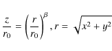
where r0 determines the ``scale of curvature'' of the bow, defined as the radius where z = r, and
The shock propagates along the z-axis with velocity
![]() into a
homogeneous medium with pre-shock density
into a
homogeneous medium with pre-shock density ![]() (
(
![]() H) + 2n(H2)) and
a uniform magnetic field.
The magnetic field
strength scales with
density as
H) + 2n(H2)) and
a uniform magnetic field.
The magnetic field
strength scales with
density as
![]()
![]() G where b is the magnetic field
scale factor.
G where b is the magnetic field
scale factor.
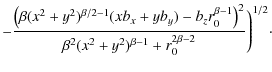
We then treat each element on the bow surface as a planar shock with local
shock
parameters. During the passage of the shock wave it is only the velocity
component perpendicular to the bow surface,
![]() ,
that contributes to the shock and transforms bulk kinetic energy into
thermal energy. Thus, the effective local shock velocity is
,
that contributes to the shock and transforms bulk kinetic energy into
thermal energy. Thus, the effective local shock velocity is
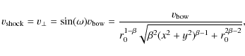
|
(2) |
where
The magnetic field acts to cushion the shock and to decouple the ions from the neutral fluid (Draine 1980). We assume that the effective
field of oblique shocks is the field component parallel to the shock surface (Smith 1992).
Thus
![]() ,
where
,
where
![]() is the local value of the
magnetic field scale factor as defined above and
is the local value of the
magnetic field scale factor as defined above and

2.2 1D shock model calculations
The planar shocks are calculated using the model described in
Flower & Pineau des Forêts (2003). This model involves, as mentioned above, a very detailed
treatment of the chemistry and
of the atomic and molecular excitation and associated cooling. Chemical events,
described by 1065 chemical processes involving 136 species, determine critical
parameters such as the degree of ionisation in the medium.
Elemental abundances are solar and are distributed among gas phase, grain
cores and grain icy mantles following Flower & Pineau des Forêts (2003). Initial
species abundances in the gas phase are derived from a steady state
calculation with a standard H2 cosmic ray ionisation rate of
![]() s-1 per H atom. This determines in particular the ratio of atomic
to molecular hydrogen and the ionisation fraction in the preshock gas.
The PAH abundance is set to
s-1 per H atom. This determines in particular the ratio of atomic
to molecular hydrogen and the ionisation fraction in the preshock gas.
The PAH abundance is set to
![]() /
/
![]() .
This has important consequences for the magnetosonic speed of the charged
fluid and therefore the maximum velocity we can achieve in C-type shocks
(Flower & Pineau des Forêts 2003, see below).
.
This has important consequences for the magnetosonic speed of the charged
fluid and therefore the maximum velocity we can achieve in C-type shocks
(Flower & Pineau des Forêts 2003, see below).
A total of 100 rovibrational level populations of H2 are calculated in parallel with the dynamical and chemical variables, allowing for all radiative transitions and collisional processes which modify level populations. This includes all relevant rotationally and rovibrationally inelastic collisions with H, He, H2 and electrons and level by level collisional dissociation, as a function of temperature (Le Bourlot et al. 2002). In dissociative shocks H2 is assumed to be reformed with an energy distribution proportional to a Boltzman distribution at 17 249 K.
Above a critical shock velocity,
![]() ,
the shock becomes a J-type
shock. The critical
velocity is defined as the minimum of
,
the shock becomes a J-type
shock. The critical
velocity is defined as the minimum of
![]() and
and
![]() ,
where
,
where
![]() is the velocity at which H2 starts to dissociate (Le Bourlot et al. 2002) and
is the velocity at which H2 starts to dissociate (Le Bourlot et al. 2002) and
![]() is the magnetosonic speed of the charged fluid. At shock velocities
higher than
is the magnetosonic speed of the charged fluid. At shock velocities
higher than
![]() the ionic precursor cannot develop ahead of the
perturbance (Flower & Pineau des Forêts 2003).
the ionic precursor cannot develop ahead of the
perturbance (Flower & Pineau des Forêts 2003).
![]() is approximately equal to the Alfven
speed in the charged fluid,
is approximately equal to the Alfven
speed in the charged fluid,
![]() ,
where
,
where
![]() is dominated by the grains and is
limited by the PAH abundance (Flower & Pineau des Forêts 2003).
is dominated by the grains and is
limited by the PAH abundance (Flower & Pineau des Forêts 2003).
![]() depends on the pre-shock density and
magnetic field strength.
The greater the component of the magnetic flux perpendicular to the direction
of propagation of the shock, the higher is the maximum
velocity at which a C-type shock can be sustained.
depends on the pre-shock density and
magnetic field strength.
The greater the component of the magnetic flux perpendicular to the direction
of propagation of the shock, the higher is the maximum
velocity at which a C-type shock can be sustained.
![]() tends to
decrease at higher density owing to the more efficient H2 dissociation.
tends to
decrease at higher density owing to the more efficient H2 dissociation.
Given the pre-shock density,
![]() ,
and
,
and
![]() ,
we
determine for each planar shock whether it is a J-type or a C-type shock.
The bow
may have a dissociative J-shock cap with oblique C-shocks along the wings as
in Fig. 1, but if
,
we
determine for each planar shock whether it is a J-type or a C-type shock.
The bow
may have a dissociative J-shock cap with oblique C-shocks along the wings as
in Fig. 1, but if ![]() is not aligned with the bow axis
the minimum of
is not aligned with the bow axis
the minimum of
![]() will be located
somewhere along the wings and
the combination of
will be located
somewhere along the wings and
the combination of ![]() and
and
![]() may result in J-type shocks
at that location. Thus, dissociative J-type shocks are not spatially
restricted to the apex.
Switch-on shocks that might exist when the angle between the shock normal and
may result in J-type shocks
at that location. Thus, dissociative J-type shocks are not spatially
restricted to the apex.
Switch-on shocks that might exist when the angle between the shock normal and
![]() approaches zero (Smith 1992; Draine & McKee 1993), that is
approaches zero (Smith 1992; Draine & McKee 1993), that is
![]() ,
have not been treated. When
,
have not been treated. When
![]() ,
the planar
shock is always a J-type shock in our model.
,
the planar
shock is always a J-type shock in our model.
2.3 Cooling distance perpendicular and parallel to the bow
We treat the shock width as resolved when constructing the 3D model.
That is, we include the distance travelled by each parcel of gas as
the gas cools, which determines the local thickness of the bow shell.
This is necessary for C-shocks which are much wider than J-shocks.
The shock width is mainly determined by the pre-shock density (see
Fig. 8 in Kristensen et al. 2007), with the width changing from a few AU at
![]() cm-3 to
cm-3 to ![]() 1000 AU at
1000 AU at
![]() cm-3. The magnetic
field scaling factor, b, also has an impact on the shock width although not as
drastic. Increasing b and thus the magnetic field naturally increases the
shock width by introducing a greater magnetic cushioning effect.
cm-3. The magnetic
field scaling factor, b, also has an impact on the shock width although not as
drastic. Increasing b and thus the magnetic field naturally increases the
shock width by introducing a greater magnetic cushioning effect.
We take into account not only the 1D cooling distance
in the shock direction, but also the distance travelled by the cooling gas
parallel to the shock front (in the bow reference frame).
In the oblique bow wings, the latter distance is greater than the 1D cooling
distance in the shock direction. This is done in an approximate way by noting that in C-shocks, the bulk of H2 rovibrational emission, which is emitted at temperatures T > 1000 K, occurs
at
velocities close to ![]() ,
before the gas has had time to slow down
by more than a few km s-1. Thus, to build our emission maps, we assume
here that the cooling gas behind each 1D shock is displaced exactly along the
z-axis
until
,
before the gas has had time to slow down
by more than a few km s-1. Thus, to build our emission maps, we assume
here that the cooling gas behind each 1D shock is displaced exactly along the
z-axis
until
![]() K. For the purpose of computing centroid velocities we
retain the exact velocity vector.
We also neglect the transverse pressure gradients and
expansion due to the bow curvature, with respect to the compressive term
included in the 1D shock models.
The accuracy of both approximations is analysed in Appendix A
for various B-field strength and preshock densities. Note that this z-axis
approximation would not be as accurate for pure rotational emission, which is
significant to lower T.
K. For the purpose of computing centroid velocities we
retain the exact velocity vector.
We also neglect the transverse pressure gradients and
expansion due to the bow curvature, with respect to the compressive term
included in the 1D shock models.
The accuracy of both approximations is analysed in Appendix A
for various B-field strength and preshock densities. Note that this z-axis
approximation would not be as accurate for pure rotational emission, which is
significant to lower T.
2.4 Intensity and centroid velocity maps
When all the resolved planar shocks are in place in the 3D model we rotate the bow by the inclination angle, i, and project it onto the 2D plane. This yields an image of the bow shock as it would appear in the plane of the sky. In performing this projection we make use of the fact that H2 emission is optically thin for any relevant column densities, since the IR quadrupole rovibrational transitions involved are weak.
The 3D model can produce maps of any of the numerous output parameters from the planar shock simulations. Thus the morphology of shocks can for example be studied by displaying the H2 emission or emission from other species. Furthermore we can create excitation diagrams or maps of excitation temperatures by calculating maps from different H2 lines.
We can also predict the centroid velocity of the H2 emission. The
pre-shock gas
is assumed stationary relative to the observer and it is only ![]() that
affects the gas. Hence, in the frame of the observer, the
post-shock gas is expanding perpendicular to the bow surface with velocity
increasing with distance from the shock front. We construct the radial velocity
map by taking the centroid velocity along the line of sight weighted by the
local H
2 v=1-0 S(1) emissivity.
We choose radial velocity maps because the radial velocity is the observable
quantity which has been reported at 150 mas spatial resolution in
Gustafsson et al. (2003) and Nissen et al. (2007).
that
affects the gas. Hence, in the frame of the observer, the
post-shock gas is expanding perpendicular to the bow surface with velocity
increasing with distance from the shock front. We construct the radial velocity
map by taking the centroid velocity along the line of sight weighted by the
local H
2 v=1-0 S(1) emissivity.
We choose radial velocity maps because the radial velocity is the observable
quantity which has been reported at 150 mas spatial resolution in
Gustafsson et al. (2003) and Nissen et al. (2007).
In building our maps we also need to truncate the bow surface at a
maximum outer radius in order to
limit the map computing time. We set this maximum outer radius equal to
![]() pixels. Both the linear resolution and the radial extent
of our maps are then fixed by the elementary pixel size that we adopt. Two
methods of choosing the pixel size in the model have been adopted.
One approach is to use
a specific number of pixels,
pixels. Both the linear resolution and the radial extent
of our maps are then fixed by the elementary pixel size that we adopt. Two
methods of choosing the pixel size in the model have been adopted.
One approach is to use
a specific number of pixels,
![]() ,
to span the thickness of the bow
shell, i.e., the maximum cooling distance of the planar shocks along the bow.
Using this approach we can fix the ratio of the thickness to truncation radius
,
to span the thickness of the bow
shell, i.e., the maximum cooling distance of the planar shocks along the bow.
Using this approach we can fix the ratio of the thickness to truncation radius
![]() of the bow shell, at the expense of letting the size of the bow shock
vary. The other approach is to fix the pixel size to a specific value. In this
approach
of the bow shell, at the expense of letting the size of the bow shock
vary. The other approach is to fix the pixel size to a specific value. In this
approach
![]() varies freely and is determined by the local shock
width. Using this method we fix the map resolution and the maximum size of the bow
shock,
varies freely and is determined by the local shock
width. Using this method we fix the map resolution and the maximum size of the bow
shock,
![]() ,
but not the relative thickness to radius. In
Sect. 3.1 we show
examples of both approaches. Otherwise, for the rest of
Sect. 3 we have used the second approach and fixed the
pixel size to 5.2 AU. In all predictions, the radius of curvature
r0 defined in Eq. (1) is 200 pixels, i.e. 1.4
,
but not the relative thickness to radius. In
Sect. 3.1 we show
examples of both approaches. Otherwise, for the rest of
Sect. 3 we have used the second approach and fixed the
pixel size to 5.2 AU. In all predictions, the radius of curvature
r0 defined in Eq. (1) is 200 pixels, i.e. 1.4
![]() ,
except in
Fig. 4 where it is 71 pixels = 0.5
,
except in
Fig. 4 where it is 71 pixels = 0.5
![]() .
.
![\begin{figure}
\par\includegraphics[width=15.8cm,clip]{12977fg2cmjn.eps}
\vspace*{-1mm}
\end{figure}](/articles/aa/full_html/2010/05/aa12977-09/img64.png)
|
Figure 2:
Brightness in Wm-2 sr-1, size and thickness in AU
of a series of shocks as a
function of pre-shock
density.
From top to bottom, the pre-shock density is
106, 105, 104 cm-3.
The shock is seen edge-on,
|
| Open with DEXTER | |
3 Model predictions
In this section we present predicted bow shock maps by exploring
the effects of the individual input parameters on the models. The input
parameters can be divided into two groups. The first group, consisting of the
pre-shock density, ![]() ,
the bow velocity,
,
the bow velocity,
![]() ,
and the magnetic field
strength, b,
determines in broad terms the brightness and the thickness of the
bow shell. The second
group regulates, again broadly, the morphology of the bow shock. This
group consists of the orientation of the magnetic field
,
and the magnetic field
strength, b,
determines in broad terms the brightness and the thickness of the
bow shell. The second
group regulates, again broadly, the morphology of the bow shock. This
group consists of the orientation of the magnetic field
![]() (Fig. 1) which fixes the
position of the most strongly emitting shocks on the bow surface and
the degree of asymmetry of the map, the angle
of inclination, i, which influences the line of sight projection, and the
geometrical parameters, r0 and
(Fig. 1) which fixes the
position of the most strongly emitting shocks on the bow surface and
the degree of asymmetry of the map, the angle
of inclination, i, which influences the line of sight projection, and the
geometrical parameters, r0 and ![]() ,
which determine the
curvature of the bow surface and thus how fast the shock conditions vary along
the wings (Eqs. (1)-(3)).
,
which determine the
curvature of the bow surface and thus how fast the shock conditions vary along
the wings (Eqs. (1)-(3)).
The effects of the groups of parameters cannot be entirely separated. It is, however, instructive at first to view them as two separate groups. In reality, the pre-shock density, the bow velocity, and the magnetic field strength will also influence the morphology of the shock since they determine the shell thickness. However the most significant effect on the shape stems from the orientation of the magnetic field and the inclination angle. On the other hand, the orientation of the magnetic field and the inclination angle also influence the brightness due to projection effects, but to a lesser degree than pre-shock density, the bow velocity, and the magnetic field strength, that is, the first group of input parameters.
In the following we first explore the effects on brightness and shell
thickness of the first group of input parameters. Then we illustrate how the
second group of parameters changes the morphology of the bow shocks. We keep
![]() constant at
constant at ![]() and give a few examples of the effect of the
r0 parameter.
and give a few examples of the effect of the
r0 parameter.
Unless otherwise stated, we use the emission from the H2 v=1-0 S(1) line
at 2.1218 ![]() m to
illustrate the morphology of the projected shocks. This is the strongest NIR
rovibrational line of
H2 and numerous shocked environments have been mapped in this line with
high spatial resolution.
In all figures brightnesses are given in Wm-2 sr-1 and sizes in AU.
m to
illustrate the morphology of the projected shocks. This is the strongest NIR
rovibrational line of
H2 and numerous shocked environments have been mapped in this line with
high spatial resolution.
In all figures brightnesses are given in Wm-2 sr-1 and sizes in AU.
3.1 Density
We start out by investigating the effect of the pre-shock density on shock
size and appearance in Fig. 2. The pre-shock density is varied
between
104-106 cm-3 while the other input parameters are kept constant
at
![]() km s-1, b=5,
km s-1, b=5,
![]() .
The input
parameters are chosen to resemble the physical conditions of OMC1 as found by
Kristensen et al. (2008) by 2D shock modelling.
The figure consists of two parts.
In the left-hand column we fix the pixel size to 1/100 of
the maximum cooling distance of the associated planar shocks so that our
bow truncation radius is 1.4 times the cooling length.
The relative thickness to size of the bow is
thus the same in all three models, and the thickness is also small compared to
the
radius of curvature r0 taken here as
.
The input
parameters are chosen to resemble the physical conditions of OMC1 as found by
Kristensen et al. (2008) by 2D shock modelling.
The figure consists of two parts.
In the left-hand column we fix the pixel size to 1/100 of
the maximum cooling distance of the associated planar shocks so that our
bow truncation radius is 1.4 times the cooling length.
The relative thickness to size of the bow is
thus the same in all three models, and the thickness is also small compared to
the
radius of curvature r0 taken here as
![]() Since the shock width decreases with increasing density
(see also Kristensen et al. 2007) the pixel size and the size of the
bow shocks are determined by
the pre-shock density.
The pixel size decreases from 142 AU at
Since the shock width decreases with increasing density
(see also Kristensen et al. 2007) the pixel size and the size of the
bow shocks are determined by
the pre-shock density.
The pixel size decreases from 142 AU at
![]() cm-3, to 27.5 AU
at
cm-3, to 27.5 AU
at
![]() cm-3 and to 5.2 AU in the
cm-3 and to 5.2 AU in the
![]() cm-3 model. The bow truncation radius is 140 times larger.
The peak brightness in the bow shock
increases with increasing density and the emission in the
wings becomes relatively stronger at high densities compared
to the apex brightness. This arises because a change in the shock velocity in
high density systems has a smaller effect on the brightness of the v=1-0 S(1)
line than at low densities. At high densities, lower J and v levels may become
more nearly thermalized and increasing the shock velocity leads to population
spread among a greater range of levels (Kristensen et al. 2007).
cm-3 model. The bow truncation radius is 140 times larger.
The peak brightness in the bow shock
increases with increasing density and the emission in the
wings becomes relatively stronger at high densities compared
to the apex brightness. This arises because a change in the shock velocity in
high density systems has a smaller effect on the brightness of the v=1-0 S(1)
line than at low densities. At high densities, lower J and v levels may become
more nearly thermalized and increasing the shock velocity leads to population
spread among a greater range of levels (Kristensen et al. 2007).
In the right-hand column of Fig. 2 we have fixed
the pixel size to 41.5 AU and thus fixed
the outer truncation radius and the curvature radius of the
bow shock to the same values of
![]() AU and
r0 = 8300 AU,
respectively, in all three models. Thus,
the relative thickness to radius of the bow shell varies due to variations of
shock width. At
AU and
r0 = 8300 AU,
respectively, in all three models. Thus,
the relative thickness to radius of the bow shell varies due to variations of
shock width. At
![]() cm-3 the shock width is very large compared
to the radius of curvature and the bow structure is hardly visible.
At
cm-3 the shock width is very large compared
to the radius of curvature and the bow structure is hardly visible.
At
![]() cm-3 the bow shell is thin and the bow structure is clear. And at
cm-3 the bow shell is thin and the bow structure is clear. And at
![]() cm-3 the shock width is so small that it is barely resolved using
the pixel size adopted.
From Fig. 2 it is clear that the appearance of a bow shock
changes dramatically if the ratio of the shock width to bow radius changes.
cm-3 the shock width is so small that it is barely resolved using
the pixel size adopted.
From Fig. 2 it is clear that the appearance of a bow shock
changes dramatically if the ratio of the shock width to bow radius changes.
In observational data the pre-shock density can be estimated by studying the width of the emitting region as well as the brightness. This has been discussed at length in Kristensen et al. (2008) in which, in 2D models, the observed shock width was found to be a valuable constraint on the physical conditions.
3.2 Bow velocity
![\begin{figure}
\par\includegraphics[width=8.5cm,clip]{12977fg3cmjn.eps}
\end{figure}](/articles/aa/full_html/2010/05/aa12977-09/img69.png)
|
Figure 3:
Brightness, size and morphology as a function of bow velocity. From
top to bottom the velocity is 60, 50, 40, and 30 km s-1. The shock is seen edge-on,
|
| Open with DEXTER | |
Figure 3 shows the effect of changing the bow shock
velocity,
![]() .
Here b,
.
Here b, ![]() ,
,
![]() ,
and r0 are kept
constant. The bow shock gets brighter when the propagation velocity is
increased. In addition a larger part of the wings contributes to the
emission. The model with
,
and r0 are kept
constant. The bow shock gets brighter when the propagation velocity is
increased. In addition a larger part of the wings contributes to the
emission. The model with
![]() km s-1 illustrates the result when the
velocity increases beyond the critical velocity for which C-shocks can be
sustained. When the velocity at the apex is higher than the critical velocity
for the given density and B-field, J-shocks are present at the apex. Thus we
have a dissociative cap with very little H2 emission. The C-shocks along the
wings
are bright and due to projection effects H2 emission is found everywhere in
the inner region behind the apex. Only the apex region itself shows weak H2emission.
km s-1 illustrates the result when the
velocity increases beyond the critical velocity for which C-shocks can be
sustained. When the velocity at the apex is higher than the critical velocity
for the given density and B-field, J-shocks are present at the apex. Thus we
have a dissociative cap with very little H2 emission. The C-shocks along the
wings
are bright and due to projection effects H2 emission is found everywhere in
the inner region behind the apex. Only the apex region itself shows weak H2emission.
3.3 Magnetic field scaling factor
In Fig. 4 we see the effect of changing the numerical value of
the magnetic scaling factor b, while keeping the other parameters constant at
![]() cm-3,
cm-3,
![]() km s-1,
km s-1,
![]() ,
and r0 = 71 pixels = 0.5
,
and r0 = 71 pixels = 0.5
![]() AU.
When b increases, the shock width increases while
the H2 brightness decreases.
This arises because the magnetic pressure is higher.
The shock
dissipation and the thermal energy production are therefore spread over a
greater distance resulting in a larger extent of the
H2 emission zone and a lower temperature and excitation (see e.g. Draine 1980).
When b=1, the shock at the apex exceeds the maximum allowed speed
for a C-shock at the chosen value of
AU.
When b increases, the shock width increases while
the H2 brightness decreases.
This arises because the magnetic pressure is higher.
The shock
dissipation and the thermal energy production are therefore spread over a
greater distance resulting in a larger extent of the
H2 emission zone and a lower temperature and excitation (see e.g. Draine 1980).
When b=1, the shock at the apex exceeds the maximum allowed speed
for a C-shock at the chosen value of
![]() cm-3and the bow apex has a dissociative cap with little H2 emission as in
Fig. 3 for 60 km s-1.
The C-shocks along the wings are very narrow with shock widths
of 24 AU. They are just resolved at the chosen pixel scale
(5.2 AU). The
critical velocity of C-shocks increases when they are embedded in
stronger
magnetic fields. Therefore, there are no dissociative caps in the
models with
b=5 and b=8. The shock width - as defined as the region where the temperature
is >1000 K - at the apex is 258 AU in the b=5 model.
At b=8 the
shock width at the apex increases to 305 AU and the wing emission
is weak since the effect of the shock wave is damped substantially by the high
magnetic field. At higher magnetic fields, the bow shock is relatively thicker
and the emission, while weaker,
is relatively more concentrated toward the symmetry axis and apex region.
cm-3and the bow apex has a dissociative cap with little H2 emission as in
Fig. 3 for 60 km s-1.
The C-shocks along the wings are very narrow with shock widths
of 24 AU. They are just resolved at the chosen pixel scale
(5.2 AU). The
critical velocity of C-shocks increases when they are embedded in
stronger
magnetic fields. Therefore, there are no dissociative caps in the
models with
b=5 and b=8. The shock width - as defined as the region where the temperature
is >1000 K - at the apex is 258 AU in the b=5 model.
At b=8 the
shock width at the apex increases to 305 AU and the wing emission
is weak since the effect of the shock wave is damped substantially by the high
magnetic field. At higher magnetic fields, the bow shock is relatively thicker
and the emission, while weaker,
is relatively more concentrated toward the symmetry axis and apex region.
![\begin{figure}
\par\includegraphics[width=8cm,clip]{12977fg4cmjn.eps}
\end{figure}](/articles/aa/full_html/2010/05/aa12977-09/img72.png)
|
Figure 4:
Brightness and thickness as a function of the magnetic field scaling
factor, b. From top to bottom, b = 8, 5, and 1. The shock is seen edge-on,
|
| Open with DEXTER | |
The effect of the curvature radius r0 may be seen by comparing the
model with b =5 in the middle panel of Fig. 4, where
![]() AU to
the model with
AU to
the model with
![]() cm-3 in
Fig. 2 left column, where
cm-3 in
Fig. 2 left column, where
![]() AU.
r0 is the only parameter that
differs between the two models. When r0 is smaller (Fig. 4
middle panel) the bow structure is narrower and the strength of the shocks
decreases faster along the wings. In fact, reducing r0 is equivalent to shrinking the bow,
with all shock parameters remaining the same.
AU.
r0 is the only parameter that
differs between the two models. When r0 is smaller (Fig. 4
middle panel) the bow structure is narrower and the strength of the shocks
decreases faster along the wings. In fact, reducing r0 is equivalent to shrinking the bow,
with all shock parameters remaining the same.
3.4 Direction of magnetic field with respect to shock propagation
![\begin{figure}
\par\includegraphics[width=15cm,clip]{12977fg5cmjn.eps}
\end{figure}](/articles/aa/full_html/2010/05/aa12977-09/img75.png)
|
Figure 5:
Left: morphology change as a function of the magnetic
field direction |
| Open with DEXTER | |
We now turn to the second group of input parameters and show how the direction
of the magnetic field with respect to the flow direction affects the
morphology of the H2 emission from a
bow shock.
The direction of the magnetic field is fixed by two angles:
the ``obliquity'' ![]() ,
defined so that
,
defined so that
![]() is the angle of B from the z-axis,
and the ``rotation'' angle
is the angle of B from the z-axis,
and the ``rotation'' angle ![]() of the projection of B on the x-y plane (see
Fig. 1).
of the projection of B on the x-y plane (see
Fig. 1).
The obliquity angle ![]() of the magnetic field with respect to the bow shock axis
has a large impact on the 3-dimensional as well as the
projected morphology. This is due to the variation
of
of the magnetic field with respect to the bow shock axis
has a large impact on the 3-dimensional as well as the
projected morphology. This is due to the variation
of
![]() across the bow profile.
When the direction of the bow propagation is at an angle to the direction of
the B-field, then one side of the bow will experience a
across the bow profile.
When the direction of the bow propagation is at an angle to the direction of
the B-field, then one side of the bow will experience a
![]() which is
different from that on the opposite side of the bow. On the side which faces
into the direction of the B-field, the value of
which is
different from that on the opposite side of the bow. On the side which faces
into the direction of the B-field, the value of
![]() will be lower than on the
opposite side. This results in brighter, thinner shocks than on the
opposite side of the bow, introducing an asymmetry in the brightness
distribution.
will be lower than on the
opposite side. This results in brighter, thinner shocks than on the
opposite side of the bow, introducing an asymmetry in the brightness
distribution.
In Appendix B, the changing morphology is illustrated in
detail. There, the standard model (
![]() cm3,
cm3,
![]() km s-1, b=5,
km s-1, b=5,
![]() AU) is displayed at six angles of
inclinations, four
different values of
AU) is displayed at six angles of
inclinations, four
different values of ![]() and seven values of
and seven values of
![]() (see Fig. 1). Here we discuss a limited number of examples
and refer to
Appendix B for a more extensive view.
Note that models with
(see Fig. 1). Here we discuss a limited number of examples
and refer to
Appendix B for a more extensive view.
Note that models with ![]() and
and
![]() are
identical under reflection in the 2nd axis of the
images, except for
are
identical under reflection in the 2nd axis of the
images, except for
![]() at certain inclinations (see below).
at certain inclinations (see below).
The left column of Fig. 5 illustrates the effect of changing the angle ![]() in our standard bow shock model, that is, with
in our standard bow shock model, that is, with
![]() cm3,
cm3,
![]() km s-1, b=5,
km s-1, b=5,
![]() AU. Here the inclination is
AU. Here the inclination is
![]() and
and
![]() (ie. magnetic field in the x-z plane). When
(ie. magnetic field in the x-z plane). When
![]() (bottom panel), the
B-field is perpendicular to the shock propagation axis and since
(bottom panel), the
B-field is perpendicular to the shock propagation axis and since
![]() the value of
the value of
![]() is symmetric with respect to the yz-plane. The projected emission from
the bow shock is therefore symmetric across x=0. When
is symmetric with respect to the yz-plane. The projected emission from
the bow shock is therefore symmetric across x=0. When
![]() (exemplified by
(exemplified by
![]() and
and
![]() ,
middle panels
of Fig. 5), the projected B-field runs from lower-left to
upper-right of the image, therefore
,
middle panels
of Fig. 5), the projected B-field runs from lower-left to
upper-right of the image, therefore
![]() is lower on the negative side of the x-axis, where the
inclined B-field is more perpendicular to the bow surface, than on the
positive side. Thus, the planar shocks and the resulting emission are
strongest on the left-hand-side in the figure and the
bow shock appears asymmetric. An extreme example may be found for the model
with
is lower on the negative side of the x-axis, where the
inclined B-field is more perpendicular to the bow surface, than on the
positive side. Thus, the planar shocks and the resulting emission are
strongest on the left-hand-side in the figure and the
bow shock appears asymmetric. An extreme example may be found for the model
with
![]() .
A ``hole''
with little H2 emission is found along a part of the wing (projected into
the region around (-300 AU, 100 AU)). This is where the B-field is
close to perpendicular to the shock surface and
.
A ``hole''
with little H2 emission is found along a part of the wing (projected into
the region around (-300 AU, 100 AU)). This is where the B-field is
close to perpendicular to the shock surface and
![]() .
The planar shocks
are therefore J-type shocks which are associated here with much weaker H2emission than C-shocks
.
The planar shocks
are therefore J-type shocks which are associated here with much weaker H2emission than C-shocks![]() .
When
.
When
![]() (top panel of Fig. 5),
the B-field is parallel to the bow axis,
and the apex region is inhabited by dissociative J-shocks with weak emission,
producing a hole towards (0, 0) in the image.
The distribution of
(top panel of Fig. 5),
the B-field is parallel to the bow axis,
and the apex region is inhabited by dissociative J-shocks with weak emission,
producing a hole towards (0, 0) in the image.
The distribution of
![]() is now
axisymmetric about the bow axis. However, due to the bow inclination of 50
is now
axisymmetric about the bow axis. However, due to the bow inclination of 50![]() to the line of
sight and the resulting limb-brightening, the projected brightness distribution is not axisymmetric
about (0, 0) and the H2 emission peak appears projected ahead of the apex.
to the line of
sight and the resulting limb-brightening, the projected brightness distribution is not axisymmetric
about (0, 0) and the H2 emission peak appears projected ahead of the apex.
Figure 5 clearly shows that dissociative J-shocks are not
constrained to the
apex region of a bow shock. They may also be found along the wings depending
on the direction of the magnetic field (![]() )
and the geometry of the bow
surface (
)
and the geometry of the bow
surface (![]() parameter). Another result is that the
peak brightness increases with
parameter). Another result is that the
peak brightness increases with ![]() .
This is because the value of
.
This is because the value of
![]() decreases at the apex where the highest
decreases at the apex where the highest
![]() is
found and the associated planar shocks become stronger.
The models in
Fig. 5 can be seen at other inclinations in Appendix B.
is
found and the associated planar shocks become stronger.
The models in
Fig. 5 can be seen at other inclinations in Appendix B.
The effect of changing the ``rotation'' angle ![]() can be seen in Fig. 6 for
which
can be seen in Fig. 6 for
which
![]() .
This corresponds to rotating the bow with respect
to the observer, without changing the overall 3D distribution of
.
This corresponds to rotating the bow with respect
to the observer, without changing the overall 3D distribution of
![]() and shock brightness on the bow surface (fixed by
and shock brightness on the bow surface (fixed by ![]() ).
).
The case
![]() (3rd panel from top) is the same as discussed
in Fig. 5: the emission is strongest to the left from the
observer's viewpoint, where x is
negative in Fig. 1. As
(3rd panel from top) is the same as discussed
in Fig. 5: the emission is strongest to the left from the
observer's viewpoint, where x is
negative in Fig. 1. As ![]() becomes negative, the B-field
rotates in towards the observer, while the strongest planar shocks
(
becomes negative, the B-field
rotates in towards the observer, while the strongest planar shocks
(
![]() lowest) rotate back to the bow side facing away from the
observer.
They experience more limb-brightening, since the rear part of the bow is more
tangential to the line of sight. When
lowest) rotate back to the bow side facing away from the
observer.
They experience more limb-brightening, since the rear part of the bow is more
tangential to the line of sight. When
![]() ,
the B-field is in
the yz-plane and points towards the observer, therefore
the emission is symmetric with respect to x=0 and is
strongly limb-brightened. In contrast, when
,
the B-field is in
the yz-plane and points towards the observer, therefore
the emission is symmetric with respect to x=0 and is
strongly limb-brightened. In contrast, when ![]() is positive (bottom
panel),
the brightness decreases since the strongest emission is now on the side of
the bow shell
facing towards the observer and is thus projected onto a
larger area. Note that because of these differences in limb-brightening, maps
with
is positive (bottom
panel),
the brightness decreases since the strongest emission is now on the side of
the bow shell
facing towards the observer and is thus projected onto a
larger area. Note that because of these differences in limb-brightening, maps
with
![]() and
and
![]() are not identical at
inclinations different from edge-on (except if
are not identical at
inclinations different from edge-on (except if
![]() or
or
![]() ),
as shown in Appendix B.
),
as shown in Appendix B.
![\begin{figure}
\par\includegraphics[width=8cm,clip]{12977fg6cmjn.eps}
\end{figure}](/articles/aa/full_html/2010/05/aa12977-09/img82.png)
|
Figure 6:
Morphology change as a function of the magnetic field direction
angle |
| Open with DEXTER | |
3.5 Inclination
![\begin{figure}
\par\includegraphics[width=7cm,clip]{12977fg7cmjn.eps}
\end{figure}](/articles/aa/full_html/2010/05/aa12977-09/img83.png)
|
Figure 7:
Morphology change as a function of the inclination angle, i. From
top to bottom,
|
| Open with DEXTER | |
The projected morphology of a bow shock naturally also depends on the angle at
which it moves with respect to the observer. Figure 7 displays
our standard shock with parameters
![]() cm3,
cm3,
![]() km s-1, b=5,
km s-1, b=5,
![]() AU,
AU,
![]() ,
,
![]() at four different inclinations. The apparent aspect ratio
of the dimensions of the shock changes significantly when the inclination
changes. The emitting region becomes broader as the inclination angle
decreases.
When the shock is seen edge-on (
at four different inclinations. The apparent aspect ratio
of the dimensions of the shock changes significantly when the inclination
changes. The emitting region becomes broader as the inclination angle
decreases.
When the shock is seen edge-on (
![]() )
the bow structure is very
apparent and the apex is clearly distinguishable by a narrow ridge of strong
emission. As the inclination decreases the strong emission ridge gradually
disappears. At
)
the bow structure is very
apparent and the apex is clearly distinguishable by a narrow ridge of strong
emission. As the inclination decreases the strong emission ridge gradually
disappears. At
![]() the strong emission region is more circular and
it is distinct from the projected boundary of the bow shock. At
the strong emission region is more circular and
it is distinct from the projected boundary of the bow shock. At
![]() the bow shock is seen face-on and the peak emission is located in the centre
of the emission region. The brightness increases when the inclination
increases because the line of sight
traverses a larger number of parcels containing post-shock gas.
the bow shock is seen face-on and the peak emission is located in the centre
of the emission region. The brightness increases when the inclination
increases because the line of sight
traverses a larger number of parcels containing post-shock gas.
From Figs. 5-7, as well as from the numerous
examples shown in Appendix B, it should be evident that the
direction of the magnetic field and the inclination to the line of sight
have a very marked influence on both the morphology of a bow shock and its
appearance to the observer. Small changes in the
angles of magnetic field with respect to shock propagation can lead to very
different shapes and bow shocks with the same intrinsic
shape can produce a large number of different observable emission
morphologies.
The peak emission may not necessarily be associated with the apex of the
bow shock. The peak can be located in front of the projected apex as in
Fig. 5 (top left) or displaced along the projected wing as in
Fig. 6 (second from top). The combination of
![]() and idetermines the exact location.
For a full exploration of
and idetermines the exact location.
For a full exploration of
![]() and i we again refer to
Appendix B.
and i we again refer to
Appendix B.
We therefore reach an important conclusion. A menagerie of shapes of shocked H2 emitting regions greets the observer in Orion and elsewhere. This is nicely exemplified by the very high spatial resolution data for OMC1 presented in Lacombe et al. (2004) obtained with the VLT/NACO adaptive optics system. In images presented there and elsewhere (e.g. Nissen et al. 2007) the presence of rounded structures which are not at all of bow form, quite symmetric bow-like forms and asymmetric or highly asymmetric but roughly bow-like forms are encountered. This variety of shapes can be attributed very largely to the phenomena which we describe here. Thus broadly speaking we can state that the somewhat confused appearance of shocked zones could be due to shocks moving at a variety of angles to the observer and to the direction the magnetic field. This arises rather naturally in a large cone-angle outflow from a massive star-forming region such as OMC1.
3.6 H2 emission line ratios
Observationally, the H2 v=2-1 S(1) line is often used together with the v=1-0 S(1) line to infer the excitation temperature and hence the shock conditions. The two lines are the brightest H2 lines from the v=2-1 and v=1-0 vibrational bands, respectively, and hence the easiest to observe.
In the planar shock models the H2 v=2-1 S(1) line peaks further downwind than the v=1-0 S(1) line and is emitted in a thinner layer because the excitation to the upper level takes place over more restricted physical conditions (Kristensen et al. 2007). This means that the ratio of 2-1 S(1) to 1-0 S(1) emission changes across the bow shell and that projection effects can further alter the relative distribution. Thus a range of values of the line ratio will be present in every model.
In the right column of Fig. 5
we show the line ratio corresponding to the models in the left column. These
differ only by the direction of the magnetic field. The
first thing to notice is that the line ratio changes significantly between the
four models and that a large range of values is associated with any
particular model. In the model with
![]() the line ratio ranges
between 0.02 and 0.069, whereas the line ratio varies between 0.02 and 0.51
when
the line ratio ranges
between 0.02 and 0.069, whereas the line ratio varies between 0.02 and 0.51
when
![]() .
At the peak of v=1-0 S(1) emission the line
ratio is 0.038 at
.
At the peak of v=1-0 S(1) emission the line
ratio is 0.038 at
![]() ,
0.066 at
,
0.066 at
![]() ,
and 0.13
in the
,
and 0.13
in the
![]() and
and
![]() models.
High line ratio values above 0.2 are usually only
seen in J-shock regions as is also evident in Fig. 5 -
for example around (-300 AU, 100 AU) in the
models.
High line ratio values above 0.2 are usually only
seen in J-shock regions as is also evident in Fig. 5 -
for example around (-300 AU, 100 AU) in the
![]() case - or in Photon
Dissociation Regions (PDRs). Here we see that bow shocks can give almost any
value depending on the angle of view and magnetic field orientation. The
high values are a result of both high
values of the line ratio in the
planar shock models and projection effects in the 3D model. The J-shocks in
the dissociative regions are very narrow (a few pixels in the model) and often
much weaker compared to the C-shocks that populate the rest of the
bow shock. This makes them very sensitive to line of sight projection. If the
line of sight traverses a tail of a C-shock within the bow the line ratio may
be altered significantly.
case - or in Photon
Dissociation Regions (PDRs). Here we see that bow shocks can give almost any
value depending on the angle of view and magnetic field orientation. The
high values are a result of both high
values of the line ratio in the
planar shock models and projection effects in the 3D model. The J-shocks in
the dissociative regions are very narrow (a few pixels in the model) and often
much weaker compared to the C-shocks that populate the rest of the
bow shock. This makes them very sensitive to line of sight projection. If the
line of sight traverses a tail of a C-shock within the bow the line ratio may
be altered significantly.
Secondly, we notice that the peak in line ratio is not coincident with the peak of the v=1-0 S(1) emission. The line ratio is very sensitive to the shock conditions and decreases with decreasing strength of the v=1-0 S(1) emission (Kristensen et al. 2009, in prep.). That is, the v=2-1 S(1) line emission decreases faster than the v=1-0 S(1) line emission when the shock becomes softer. Thus, the v=2-1 S(1) emission is less extended along the wings and it is emitted in a thinner layer than the v=1-0 S(1) emission. In short, it is more concentrated towards the location of strong shocks. When the bow shock is inclined to the line of sight the peak of the line ratio will be found close to the projected location of the strong shocks, whereas the peak of v=1-0 S(1) emission may be found displaced from this due to limb-brightening. For example, in Fig. 5 lower left corner, the v=1-0 S(1) emission peaks at (0 AU, -90 AU) due to limb-brightening, whereas the line ratio peaks at (0, 0), which is the projected position of the bow apex. Thus, the relative position of the peak of v=1-0 S(1) emission and the v=2-1 S(1) / v=1-0 S(1) line ratio is very useful for determining the inclination in observations of bow shocks.
3.7 Excitation temperature
![\begin{figure}
\par\includegraphics[width=7.5cm,clip]{12977fg8.ps}
\end{figure}](/articles/aa/full_html/2010/05/aa12977-09/img86.png)
|
Figure 8:
Example of an excitation diagram from the 3D model in a region where the
gas is not completely thermalized. The v=1-0 band and the v=2-1
band do not line up. Both bands are well fitted individual by the same
excitation temperature of 2600 K (dotted and dashed line,
respectively), but with an offset. If both bands are included in the
fit (full line), the resulting excitation temperature
of 1900 K is lower than if only one band is used. The input
parameters of the model are
|
| Open with DEXTER | |
![\begin{figure}
\par\includegraphics[width=8cm,clip]{12977fg9cmjn.eps}
\end{figure}](/articles/aa/full_html/2010/05/aa12977-09/img87.png)
|
Figure 9:
Excitation temperature as a function of the magnetic field
direction |
| Open with DEXTER | |
In this section we investigate the spatial variation of the excitation
temperature measured from a number of H2 lines.
The excitation temperature is the
temperature that reproduces the observed line ratios assuming local
thermodynamic equilibrium, LTE. Under LTE conditions the column density of the
level (v,J) is
where
![\begin{figure}
\par\includegraphics[angle=90,width=14.5cm,clip]{12977f10cmjn.eps}
\end{figure}](/articles/aa/full_html/2010/05/aa12977-09/img90.png)
|
Figure 10:
Centroid radial velocities as a function of inclination and
magnetic field direction. From top to bottom
|
| Open with DEXTER | |
The degree of thermalization depends on the gas density, while collisions generate local thermodynamic equilibrium and LTE is therefore more closely achieved in high density gas. Whether the gas reaches LTE also depends strongly on the density of atomic H, as it is more efficient than H2 at collisionally exciting vibrational levels. In our models the initial H/H2 ratio is fixed at a value determined by the ambient cosmic ray rate. Thermalization would be increased if the pre-shock gas was partly dissociated by previous shocks or by a far-ultraviolet field. We do not consider this possibility here to limit the number of free parameters.
We use the v=1-0 band to extract the excitation temperature
(Fig. 9) of the models displayed in Fig. 5.
In the models in Fig. 9 the excitation temperature is ![]() 2300-3300 K and the temperature is highest in the part of the bow shock
where the planar shocks are strongest. This is either at the projected
position of the apex or the part of the wings facing
toward the magnetic field. The structure of the excitation temperature is the
same as that of the v=2-1 S(1)/v=1-0 S(1) line ratio for the same reasons as
discussed for the line ratios.
In parts of the
dissociative regions, the excitation temperature is very low, which
is unexpected since J-shocks are associated with high temperatures.
The low temperature stems from the fact that we use only lines from the v=1-0band to calculate the temperature and thus effectively calculate the
rotational temperature of the v=1-0 band. In the J-shocks used here the
rotational temperature of the v=1-0 band is lower than that of the v=2-1 band
as well as the vibrational temperature, in contrast to C-shocks as discussed
above.
2300-3300 K and the temperature is highest in the part of the bow shock
where the planar shocks are strongest. This is either at the projected
position of the apex or the part of the wings facing
toward the magnetic field. The structure of the excitation temperature is the
same as that of the v=2-1 S(1)/v=1-0 S(1) line ratio for the same reasons as
discussed for the line ratios.
In parts of the
dissociative regions, the excitation temperature is very low, which
is unexpected since J-shocks are associated with high temperatures.
The low temperature stems from the fact that we use only lines from the v=1-0band to calculate the temperature and thus effectively calculate the
rotational temperature of the v=1-0 band. In the J-shocks used here the
rotational temperature of the v=1-0 band is lower than that of the v=2-1 band
as well as the vibrational temperature, in contrast to C-shocks as discussed
above.
3.8 Radial velocity structure of bow shocks
The radial velocity structure of bow shocks is of considerable interest for comparison with observational data. With integral field spectroscopy and Fabry-Perot interferometry (Gustafsson et al. 2003; Nissen et al. 2007) it is now possible to obtain 2D maps of the radial velocity of many shocked regions. The velocity information obtained from both integral field spectroscopy and slit-spectroscopy is often also utilised via position-velocity diagrams (e.g., Takami et al. 2007,2006).
We have calculated the radial
velocity as described in Sect. 2 and maps of centroid
velocities of the standard model moving at certain angles to the B-field and
line of sight are displayed in Fig. 10 for
![]() .
The blue-shifted radial velocity is naturally at a maximum when the bow shock
is viewed face-on (righthand column in Fig. 10) and the post-shock
gas from the apex is moving in the radial
direction. The shock velocity at the apex is 40 km s-1 in these models,
but the bulk of the emitting post-shock gas is moving at lower velocities of
.
The blue-shifted radial velocity is naturally at a maximum when the bow shock
is viewed face-on (righthand column in Fig. 10) and the post-shock
gas from the apex is moving in the radial
direction. The shock velocity at the apex is 40 km s-1 in these models,
but the bulk of the emitting post-shock gas is moving at lower velocities of
![]() 9-15 km s-1. The velocity of the post-shock gas is higher when
9-15 km s-1. The velocity of the post-shock gas is higher when
![]() than when
than when
![]() .
That is because
as
.
That is because
as ![]() increases, the magnetic field is closer to the bow axis
and the
increases, the magnetic field is closer to the bow axis
and the
![]() component decreases.
The shocks are thus narrower and
the hot H2 emitting gas reaches
velocities closer to the shock speed in the observer's frame.
When the shock is moving at an angle
component decreases.
The shocks are thus narrower and
the hot H2 emitting gas reaches
velocities closer to the shock speed in the observer's frame.
When the shock is moving at an angle
![]() to the line of sight the
radial velocity
decreases and the peak velocity is offset from the peak brightness.
The maximum velocity is found behind the maximum brightness within the body of
the projected bow shock.
to the line of sight the
radial velocity
decreases and the peak velocity is offset from the peak brightness.
The maximum velocity is found behind the maximum brightness within the body of
the projected bow shock.
Since we use the centroid radial velocity, where the
velocity of each parcel of gas is weighted by the corresponding emission, the
velocity structure is very dependent on the location in the line of sight of
the emitting gas and may become highly asymmetric. In Fig. 10,
![]() .
Therefore, when
.
Therefore, when
![]() the emission is brighter
(lower b
the emission is brighter
(lower b
![]() )
on the left
hand quadrant of the front side of the bow.
When the bow shock is seen edge-on (left column),
the emission is therefore dominated by blue-shifted features.
In the model with
)
on the left
hand quadrant of the front side of the bow.
When the bow shock is seen edge-on (left column),
the emission is therefore dominated by blue-shifted features.
In the model with
![]() (upper left corner in Fig. 10) the
dissociative region is also located in the advancing side of the bow, but the
emission there is so weak that the C-shocks in the receding wing are found to
dominate the emission. This explains the small patch of redshifted velocities around
(-200, 100) AU inside the dominantly blueshifted region.
(upper left corner in Fig. 10) the
dissociative region is also located in the advancing side of the bow, but the
emission there is so weak that the C-shocks in the receding wing are found to
dominate the emission. This explains the small patch of redshifted velocities around
(-200, 100) AU inside the dominantly blueshifted region.
When
![]() and
and
![]() ,
the emission is equally strong in the left hand side of the advancing
wing and in the right hand side of the receding wing, and weak on the
opposite
sides. When such a bow is seen edge-on (lower left corner of Fig. 10), the projected emission map is thus symmetric and the centroid velocities
are blueshifted to the left and redshifted to the right of the axis of
propagation. This is the same structure as expected from a rotating
flow, although the structure clearly does not arise from
rotation. Rather, it arises purely from the fact that the emission from the
expanding post-shock gas in the
bow shock is not cylindrically symmetric around the propagation axis due to the
obliquity of the magnetic field from the bow axis.
This result shows that any search for rotating outflows needs to be conducted
with care and any interpretation must include the effects of the
magnetic field on the ambient medium.
A velocity change in the outflow
perpendicular to the outflow direction may be a projection effect in an
expanding outflow lighting up asymmetrically.
,
the emission is equally strong in the left hand side of the advancing
wing and in the right hand side of the receding wing, and weak on the
opposite
sides. When such a bow is seen edge-on (lower left corner of Fig. 10), the projected emission map is thus symmetric and the centroid velocities
are blueshifted to the left and redshifted to the right of the axis of
propagation. This is the same structure as expected from a rotating
flow, although the structure clearly does not arise from
rotation. Rather, it arises purely from the fact that the emission from the
expanding post-shock gas in the
bow shock is not cylindrically symmetric around the propagation axis due to the
obliquity of the magnetic field from the bow axis.
This result shows that any search for rotating outflows needs to be conducted
with care and any interpretation must include the effects of the
magnetic field on the ambient medium.
A velocity change in the outflow
perpendicular to the outflow direction may be a projection effect in an
expanding outflow lighting up asymmetrically.
4 Comparison of 1D and 3D models
The emission structure of a bow shock is determined by geometry, bow velocity, pre-shock density of the ambient material and the magnetic field. When using shock models to reproduce observational data, we are in many circumstances only interested in extracting the bow velocity, and the density of the ambient medium, because that is related to the thrust in outflows from young stars and the driving mechanism of these outflows. In this case we only need to recover the shock conditions at the apex of the bow and it might seem a little excessive to use a 3D model instead of a much simpler 1D model.
In this section, we simulate observations from long slit spectroscopy of the apparent peak of the bow shock, and spatially unresolved observations of the bow shock, in order to test whether these can be used together with 1D models to recover the simulated shock conditions convincingly. That is, we use the simulated brightness maps of a 3D bow shock to extract the H2 brightness from the apparent peak of the model as well as the average projected H2 brightness from the whole bowshock. We compare these to the H2 excitation diagram from the 1D shock at the apex of the 3D model, in which the bow shock conditions are imprinted.
We use our
standard 3D model with
![]() ,
,
![]() ,
seen at an
inclination of
,
seen at an
inclination of
![]() (see Fig. 5 lower left panel) as a
test case and extract the simulated observable brightness from this.
In Fig. 11 we compare the extracted column densities
to those of the 1D apex shock of the 3D bow model. First, we notice
that the column densities at the brightness peak of the 3D model are higher than
the column densities in the 1D apex shock by a factor of 1.5-3. The position
of the peak emission ((0, -80) AU in
Fig. 5 lower left panel) is limb brightened as the line of sight
traverses a large amount of gas in the bow wing. On the other hand, the
averaged column densities from the 3D model are lower than the column
densities in the 1D apex shock since they are
averages over the full extent of the bow shock where the brightness is greater
than 10% of the peak.
Furthermore, the column densities of the apparent apex
deviate more
from the 1D apex shock, both in terms of absolute values in the v=1-0 levels
and in the
difference between the v=1 and the v=2 levels, than the average column
density of the 3D model. We thus expect that using the average column
densities of the shocked emission to fit the initial shock conditions gives
a better match than using the peak of emission.
(see Fig. 5 lower left panel) as a
test case and extract the simulated observable brightness from this.
In Fig. 11 we compare the extracted column densities
to those of the 1D apex shock of the 3D bow model. First, we notice
that the column densities at the brightness peak of the 3D model are higher than
the column densities in the 1D apex shock by a factor of 1.5-3. The position
of the peak emission ((0, -80) AU in
Fig. 5 lower left panel) is limb brightened as the line of sight
traverses a large amount of gas in the bow wing. On the other hand, the
averaged column densities from the 3D model are lower than the column
densities in the 1D apex shock since they are
averages over the full extent of the bow shock where the brightness is greater
than 10% of the peak.
Furthermore, the column densities of the apparent apex
deviate more
from the 1D apex shock, both in terms of absolute values in the v=1-0 levels
and in the
difference between the v=1 and the v=2 levels, than the average column
density of the 3D model. We thus expect that using the average column
densities of the shocked emission to fit the initial shock conditions gives
a better match than using the peak of emission.
![\begin{figure}
\par\includegraphics[width=7cm,clip]{12977f11.ps}
\end{figure}](/articles/aa/full_html/2010/05/aa12977-09/img94.png)
|
Figure 11:
Deviations in column density of H2 levels of the 3D model with
respect to the 1D shock in the apex. The column densities of the
emission peak in the 3D model (+ -signs) are higher than those of the
1D apex shock, whereas the average column density of the 3D model is
lower (diamonds). The column densities of the emission peak deviate more
from the 1D shock, both in terms of absolute values and in the
difference between the v=1 and the v=2 levels, than the average column
density of the 3D model. The model parameters are
|
| Open with DEXTER | |
5 Reproducing observations
The real value of a 3D bow shock model is the ability to model observations realistically. The Herbig-Haro objects HH7, HH211, HH212, and HH240 have previously undergone detailed 3D modelling (Smith et al. 2007; O'Connell et al. 2005,2004; Smith et al. 2003) by means of the 3D bow shock model of Smith et al. (2003). In this section we show an example of how our 3D model can be used to model a bow shock observed at sub-arcsecond resolution in the Orion star forming region.
5.1 Observational constraints and previous modelling
The bow shock in question is found in the Orion Molecular Cloud 1, Southwest
of the BN object, Source I and the IRc2 complex. It is part of a blue-shifted
outflow system originating in the vicinity of Source I (Nissen et al. 2007, and references
therein). It is located at the coordinates 20
![]() 5
W and 6
5
W and 6
![]() S of TCC0016 (see Kristensen et al. (2008) for a finding chart) and
has previously been studied extensively. The great amount of information that
is available concerning this object constrains the outputs of the 3D
model, which makes the
object a good test case.
S of TCC0016 (see Kristensen et al. (2008) for a finding chart) and
has previously been studied extensively. The great amount of information that
is available concerning this object constrains the outputs of the 3D
model, which makes the
object a good test case.
The magnetic field strength in the OMC1 region has been inferred from several observations.
Zeeman measurements show that the magnetic field is ![]() 3 mG near IRc2 (Norris 1984) and that it is of the order of 0.3 mG 24
3 mG near IRc2 (Norris 1984) and that it is of the order of 0.3 mG 24
![]() North of IRc2 (Crutcher et al. 1999). Chrysostomou et al. (1994)
estimate the Alfven velocity by measuring the dispersion of
polarization angles tracing the magnetic field direction.
From this they find that
North of IRc2 (Crutcher et al. 1999). Chrysostomou et al. (1994)
estimate the Alfven velocity by measuring the dispersion of
polarization angles tracing the magnetic field direction.
From this they find that ![]() for a turbulent velocity of 1 km s-1.
for a turbulent velocity of 1 km s-1.
Kristensen et al. (2008,2007) have previously modelled the shock with 1D
and 2D
shock models respectively. Kristensen et al. (2007) found that a 1D shock with velocity ![]() 35-40 km s-1 and pre-shock density of
35-40 km s-1 and pre-shock density of
![]() cm-3 could
reproduce the brightness of the v=1-0 S(0) and S(1) lines. Using a 2D edge-on model
and higher resolution data to reproduce the brightness and emission width
along the bow wings, Kristensen et al. (2008) adjusted the
shock parameters to a velocity
cm-3 could
reproduce the brightness of the v=1-0 S(0) and S(1) lines. Using a 2D edge-on model
and higher resolution data to reproduce the brightness and emission width
along the bow wings, Kristensen et al. (2008) adjusted the
shock parameters to a velocity ![]() 50 km s-1, pre-shock density of
50 km s-1, pre-shock density of
![]() cm-3 and b=4.8.
This corresponds to a magnetic field strength at the apex of
cm-3 and b=4.8.
This corresponds to a magnetic field strength at the apex of ![]()
![]() mGauss.
From the variations in modelled shock velocity and magnetic field
strength along the wings of the bow shock they calculated the position angle of
the flow to be
mGauss.
From the variations in modelled shock velocity and magnetic field
strength along the wings of the bow shock they calculated the position angle of
the flow to be ![]()
![]() and the position angle of the
magnetic field to be
and the position angle of the
magnetic field to be ![]()
![]() .
From this, they concluded
that the magnetic field is oriented tangentially to the apex.
The direction of the
magnetic field is consistent with measurements of polarized light
that indicate that the magnetic field has
a position angle of
.
From this, they concluded
that the magnetic field is oriented tangentially to the apex.
The direction of the
magnetic field is consistent with measurements of polarized light
that indicate that the magnetic field has
a position angle of ![]()
![]() (e.g. Hough et al. 1986; Tamura et al. 2006; Chrysostomou et al. 1994; Simpson et al. 2006).
While the 2D model is successful in estimating the direction of the magnetic
field it is not capable of simultaneously reproducing the width of the
emission and the brightness. The width is underestimated by
(e.g. Hough et al. 1986; Tamura et al. 2006; Chrysostomou et al. 1994; Simpson et al. 2006).
While the 2D model is successful in estimating the direction of the magnetic
field it is not capable of simultaneously reproducing the width of the
emission and the brightness. The width is underestimated by ![]()
![]() for
the best conditions specified in Kristensen et al. (2008).
for
the best conditions specified in Kristensen et al. (2008).
Using the GriF FP interferometer on CFHT Nissen et al. (2007) measured radial
velocities of H2 emitting in the v =
1-0 S(1) line. They measured a peak radial velocity of -36 km s-1, that is, the object is moving towards us at ![]() km s-1. Recent proper motion studies performed by
Cunningham (2006) indicate that this object has a proper motion
of
km s-1. Recent proper motion studies performed by
Cunningham (2006) indicate that this object has a proper motion
of ![]() km s-1. The full 3D velocity of this object is
then
km s-1. The full 3D velocity of this object is
then ![]()
![]() km s-1 and the angle with respect to the line of
sight is
km s-1 and the angle with respect to the line of
sight is ![]()
![]() .
Therefore, one expects limb-brightening
effects that are not taken into account in the
2D edge-on model of Kristensen et al. (2008).
.
Therefore, one expects limb-brightening
effects that are not taken into account in the
2D edge-on model of Kristensen et al. (2008).
We use here the same data set as Kristensen et al. (2008) for the 3D modelling
(Fig. 12). These
data were obtained in Dec. 2004 at ESO-VLT with the NACO Fabry-Perot
interferometer. Scans were made of the v=1-0 S(1) and S(0) lines as well as
the v=2-1 S(1) line. The brightness of the three lines was
extracted by line-fitting for all spatial positions. The full data reduction has
been described in Gustafsson (2006) and Kristensen et al. (2008). The
spatial resolution is ![]() 0
0
![]() 13 or 60 AU at the distance of OMC1, while
the pixel size is 11 AU.
13 or 60 AU at the distance of OMC1, while
the pixel size is 11 AU.
![\begin{figure}
\par\includegraphics[angle=90,width=15.5cm,clip]{12977f12cmjn.eps}
\end{figure}](/articles/aa/full_html/2010/05/aa12977-09/img112.png)
|
Figure 12:
Brightness of a bow shock in OMC1 observed
at ESO-VLT and the corresponding radial velocity map from
Nissen et al. (2007) ( upper row) compared to the best fit 3D model ( lower row). The
observational data has been rotated clockwise by 55 |
| Open with DEXTER | |
5.2 Fitting procedure
The 3D model has 8 free parameters (see Table 1) and it is very time consuming to do a large
grid-based search of the model that best reproduces the observations if all
parameters are included. Therefore, we start by doing some manual
exploration in
order to limit the parameter space. To facilitate the comparison between
observations and model we first rotate the observations so that the
flow is moving along the z-axis as in the models. Kristensen et al. (2008)
estimated
the required rotation by fitting a parabola to the ridge of peak emission and
found that a rotation of 55![]() provided a minimum
provided a minimum ![]() value. We
adopt this result and rotate the observations clockwise by 55
value. We
adopt this result and rotate the observations clockwise by 55![]() .
Fitting a
power-law to the ridge of peak emission yields initial values of the
r0 and
.
Fitting a
power-law to the ridge of peak emission yields initial values of the
r0 and ![]() parameters of 400 AU and 1.7, respectively (see
Eq. (1)). These estimates of
r0 and
parameters of 400 AU and 1.7, respectively (see
Eq. (1)). These estimates of
r0 and ![]() assume that the bow shock is seen edge-on. Therefore
they may require later adjustment.
assume that the bow shock is seen edge-on. Therefore
they may require later adjustment.
Second, we seek to constrain the inclination
angle and the direction of the magnetic field.
The morphology of the observed flow helps to constrain the inclination. The
emission region is relatively broad with extended emission behind the apex. The
apparent apex (the location of peak emission) is, however, clearly distinguishable and
the emission falls off more quickly in front of the apex than behind.
From the results described in Sect. 3.5 and the figures in
Appendix B it is clear that extended emission behind the apex
together with a rapid decrease in emission in front limits the inclination
angle to
![]() .
As an initial value we use the inclination
angle indicated by the velocity observations of
.
As an initial value we use the inclination
angle indicated by the velocity observations of
![]() .
.
Third, we run a mini-grid of 3D models with different values of ![]() and
and
![]() ,
which define the orientation of the magnetic field with respect to the
shock motion. The goal is to find the direction of the magnetic field that
reproduces the
morphology of the observed flow, namely the location and the degree of
asymmetry of the bright emission.
We use the results of Kristensen et al. (2008) as the initial input parameters of
the
3D model. We calculate a 3D model with
,
which define the orientation of the magnetic field with respect to the
shock motion. The goal is to find the direction of the magnetic field that
reproduces the
morphology of the observed flow, namely the location and the degree of
asymmetry of the bright emission.
We use the results of Kristensen et al. (2008) as the initial input parameters of
the
3D model. We calculate a 3D model with
![]() cm-3,
cm-3,
![]() ,
b=5,
,
b=5, ![]() ,
r0=400 AU and
,
r0=400 AU and
![]() .
We explore
.
We explore
![]() ,
,
![]() ,
and
,
and
![]() and let
and let ![]() vary between
vary between
![]() and
and
![]() in steps of
in steps of
![]() .
We adopt the same pixel size as in the observation, that is, 11 AU.
.
We adopt the same pixel size as in the observation, that is, 11 AU.
In order to compare the morphology of the observations and the models we
consider only emission stronger than a third of the peak v=1-0 S(1)
emission,
![]() .
This emission level traces the asymmetry of the
emission (see Fig. 5) while
being above the noise level in the observational data.
The asymmetry of the outer boundary of the
.
This emission level traces the asymmetry of the
emission (see Fig. 5) while
being above the noise level in the observational data.
The asymmetry of the outer boundary of the
![]() emission is determined
by
emission is determined
by ![]() and
and ![]() .
By contrast the inner boundary
behind the apex is
set by the width of the planar shocks which is given by the combination of
.
By contrast the inner boundary
behind the apex is
set by the width of the planar shocks which is given by the combination of ![]() ,
,
![]() and b. For the moment we seek only to constrain
and b. For the moment we seek only to constrain ![]() and
and
![]() ,
and therefore we consider only the contour of the outer
boundary.
We calculate
the deviation between the outer boundary of the
,
and therefore we consider only the contour of the outer
boundary.
We calculate
the deviation between the outer boundary of the
![]() emission of the observations and the models in the mini-grid. The minimum
deviation is found
at
emission of the observations and the models in the mini-grid. The minimum
deviation is found
at
![]() and
and
![]() .
.
Fourth, we run a new mini-grid where ![]() ,
r0,
,
r0, ![]() ,
,
![]() and b
are varied and
and b
are varied and
![]() ,
,
![]() and
and
![]() are kept constant. The values used in the mini-grid are:
are kept constant. The values used in the mini-grid are:
We calculate both the v=1-0 S(1) and the v=2-1 S(1) emission map and fit both to the observations. The v=1-0 S(0) emission map was not used in the fit in order to reduce the computation time. This is the last step in the fitting recipe and we now seek to reproduce both the brightness of the H2 lines and the brightness distribution of the observed flow. To this end we extract five vertical slices from the observations and find the peak brightness and FWHM of the brightness profile in each slice for both the v=1-0 S(1) and the v=2-1 S(1) lines. Each slice is 5 pixels = 55 AU wide, they are separated by 3 pixels, and we place one slice on the bow axis, one to the left of the bow axis and three to the right. In the same way we slice up the models and extract peak values and FWHM of the brightness profiles. We then use a
5.3 Modelled versus observed maps
Table 1: Model parameters of the model that best reproduces the observations.
The brightness maps of the v=1-0 S(1), the v=1-0 S(0) and the v=2-1 S(1) lines from the observations, as well as the associated radial velocity map from Nissen et al. (2007) are compared to the best fit model in Figs. 12 and 13. The brightness of the model is in good agreement with the observations. The modelled brightness of the v=1-0 S(1) line is about 30% too high compared to the observations, whereas the v=2-1 S(1) brightness is underestimated by a factor of two. Note that the fit to the v=2-1 S(1) brightness could be improved by increasing the H/H2ratio. This would create more collisions and thereby LTE conditions would be more closely achieved. However, we fix the H/H2 ratio by the cosmic ray rate. This is in contrast to Smith et al. (2003) who use the H/H2 ratio as a free parameter. The v=1-0 S(0) brightness, which was not included in the fit, is onlyThe width of the shock as well as the general morphology of the flow is also very well reproduced for all three emission lines. From Fig. 13 it is evident that the observed and modelled contours of 20%, 50% and 80% of the maximum brightness agree to a great extent. The asymmetric tail of emission extending towards the upper right corner is also well reproduced by the model. The ability of the 3D model to reproduce simultaneously the brightness and the width of the emission is a substantial improvement over existing 1D and 2D shock models.
![\begin{figure}
\par\includegraphics[angle=90,width=12cm,clip]{12977f13.ps}
\end{figure}](/articles/aa/full_html/2010/05/aa12977-09/img136.png)
|
Figure 13: Contours of brightness and radial velocity from the observations (blue) and the model (red). The contour levels in the three brightness plots are 0.2, 0.5, and 0.8 times the maximum brigthness. In the plot of radial velocity the contours delineate -20, -15, -10, -5, and 0 km s-1. |
| Open with DEXTER | |
The radial velocity in the model peaks at the same position as the observed
velocities, that is, behind the apex. This is very encouraging and confirms
that at least the inclination of the model is correct. The modelled velocities
are, however, lower than the observed by ![]() 20 km s-1 towards the apex.
A possible explanation may be that the apex region contains
an additional contribution from a Mach disk,
as mentioned in Kristensen et al. (2008).
20 km s-1 towards the apex.
A possible explanation may be that the apex region contains
an additional contribution from a Mach disk,
as mentioned in Kristensen et al. (2008).
We find that the magnetic field is oriented at a small angle
![]() from the
tangential plane of the apex. This is consistent with the results in Kristensen et al. (2008), who found
that the magnetic field is tangential to the bow
apex. With
from the
tangential plane of the apex. This is consistent with the results in Kristensen et al. (2008), who found
that the magnetic field is tangential to the bow
apex. With
![]() and
and
![]() ,
we predict that the
B-field projected in the plane of the sky makes an angle of
,
we predict that the
B-field projected in the plane of the sky makes an angle of ![]() from
the bow axis, ie. a PA angle of
from
the bow axis, ie. a PA angle of
![]() from North after
correcting for the rotation applied to the bow image. This is
in excellent agreement with the results in Kristensen et al. (2008) and with
polarization measurements that indicate a
from North after
correcting for the rotation applied to the bow image. This is
in excellent agreement with the results in Kristensen et al. (2008) and with
polarization measurements that indicate a
![]() in this region
(e.g. Hough et al. 1986; Tamura et al. 2006; Chrysostomou et al. 1994; Simpson et al. 2006).
The b = 3 value of our best fit model is lower than the b = 4.8
estimated by Kristensen et al. (2008) and the scaling factor
in this region
(e.g. Hough et al. 1986; Tamura et al. 2006; Chrysostomou et al. 1994; Simpson et al. 2006).
The b = 3 value of our best fit model is lower than the b = 4.8
estimated by Kristensen et al. (2008) and the scaling factor
![]() inferred by
Chrysostomou et al. (1994), but we note that the latter was estimated in a
slightly
different region (south-east of Irc2) and could be uncertain by a factor 2.
For our pre-shock density of 105 cm-3, b = 3 corresponds to a
magnetic field strength of
inferred by
Chrysostomou et al. (1994), but we note that the latter was estimated in a
slightly
different region (south-east of Irc2) and could be uncertain by a factor 2.
For our pre-shock density of 105 cm-3, b = 3 corresponds to a
magnetic field strength of ![]() 1 mG. We then predict a line of sight
component of
1 mG. We then predict a line of sight
component of ![]() 0.16 mG for
0.16 mG for
![]() and
and
![]() .
In
comparison, Zeeman
detections range from 0.3 mG to 3 mG around Irc2
(Norris 1984; Crutcher et al. 1999).
Since bowshocks bright in H2 will tend to be found preferentially in areas
of lower
magnetic field strength, the agreement is again quite good.
.
In
comparison, Zeeman
detections range from 0.3 mG to 3 mG around Irc2
(Norris 1984; Crutcher et al. 1999).
Since bowshocks bright in H2 will tend to be found preferentially in areas
of lower
magnetic field strength, the agreement is again quite good.
Thus, with the 3D model we can simultaneously reproduce the brightness levels in three H2 lines as well as the shape and size of the emitting region. The radial velocity map of the model is in qualitative agreement with the observed. Furthermore, the predicted magnetic field direction is in excellent agreement with the observed one while the scaling factor b, and amplitude of the magnetic field appear consistent with the range of observed values.
6 Concluding remarks
We have presented a three-dimensional model of interstellar bow shocks propagating in a homogeneous molecular medium with a uniform magnetic field. The model is constructed by associating a one-dimensional planar shock with every point on a three-dimensional bow skeleton. Improvements over previous work are the inclusion of a highly sophisticated chemical reaction network, which is essential for predicting realistic emission brightness, and a (simplified) treatment of motion parallel to the bow surface.
With the 3D model we can predict the projected morphology in the plane of the sky of a bow shock moving at an arbitrary inclination and with a magnetic field inclined at an arbitrary angle. In this paper we have focussed on rovibrational molecular hydrogen emission, but emission maps of atomic species and other molecular species can also be predicted. To limit the number of free parameters, we assume here that the preshock ionization and the atomic H fraction are set by the cosmic ray flux, i.e. the preshock gas is assumed well screened from any far-ultraviolet source.
The shock width depends primarily on density, with increasingly narrower shocks for higher density. The appearance in the plane of the sky of a bow shock changes dramatically if the ratio of the shock width to the curvature of the bow shell changes. If the shock width is large compared to the local radius of curvature, the emission region is very compact and the bow structure is not discernible.
The magnetic scale factor,
![]() /
/
![]() ,
also strongly influences the shock width. When b
increases, the shocks get softer and more extended. When the propagation
velocity,
,
also strongly influences the shock width. When b
increases, the shocks get softer and more extended. When the propagation
velocity,
![]() ,
is increased the shocks become stronger and a larger part
of the wings lights up. If
,
is increased the shocks become stronger and a larger part
of the wings lights up. If
![]() is increased above the critical velocity
at which a C-shock can be sustained for the given density and b-value, a
dissociative cap inhabited by dissociative J-shocks develops.
is increased above the critical velocity
at which a C-shock can be sustained for the given density and b-value, a
dissociative cap inhabited by dissociative J-shocks develops.
The morphology of the emission from a bow shock is highly dependent on the
orientation of the magnetic field and the inclination of the flow. The planar
shocks are strongest on the part of the bow surface that faces towards the
magnetic field, where the parallel field strength
![]() is lowest.
The result is that the morphology can be highly asymmetric.
Together with inclination effects this means that bow shocks can appear in
many different guises and they do not necessarily - or even generally - show
a characteristic bow shape.
Thus broadly speaking we can state that the
somewhat confused appearance of shocked zones in star forming regions could be
due
to shocks moving at a
variety of angles to the observer and to the direction of the magnetic field.
is lowest.
The result is that the morphology can be highly asymmetric.
Together with inclination effects this means that bow shocks can appear in
many different guises and they do not necessarily - or even generally - show
a characteristic bow shape.
Thus broadly speaking we can state that the
somewhat confused appearance of shocked zones in star forming regions could be
due
to shocks moving at a
variety of angles to the observer and to the direction of the magnetic field.
J-shocks may also be found in
the part of the wing of the bow where
![]() leading to a
shock velocity in excess of the critical velocity. The molecular
hydrogen emission from dissociative shocks is often much weaker than that from
C-shocks. Thus, dissociative regions in the bow
may show up as depressions in the brightness. Depressions due to dissociative
caps at the apex, mentioned above, can appear behind a leading ridge of
emission if the bow shock is not moving in the plane of the sky.
leading to a
shock velocity in excess of the critical velocity. The molecular
hydrogen emission from dissociative shocks is often much weaker than that from
C-shocks. Thus, dissociative regions in the bow
may show up as depressions in the brightness. Depressions due to dissociative
caps at the apex, mentioned above, can appear behind a leading ridge of
emission if the bow shock is not moving in the plane of the sky.
The H2 v=2-1 S(1) line is emitted efficiently under more restricted physical conditions and therefore in a thinner layer than the v=1-0 S(1) line. The ratio of the two lines is therefore variable across the flow, and the spatial offset between the peaks of the lines may be used to estimate the inclination of the flow.
We have also computed centroid radial velocity maps of bow shocks. The radial velocity is naturally maximum when the shock is seen face-on and decreases when the inclination increases. The radial velocity peaks behind the brightest region of the bow shock when the flow is seen at an inclination different from face-on. Under certain circumstances the radial velocity of an expanding bow shock can show the same signatures as a rotating flow. In this case a velocity gradient perpendicular to the outflow direction is a projection effect of an expanding bow shock lighting up asymmetrically due to the orientation of the magnetic field.
Using the 3D model we have tested whether it is possible to infer the underlying shock conditions at the bow apex by fitting 1D models to line brightnesses extracted from the projected maps. Our results indicate that the apex shock conditions are better retrieved if the average line emission over the bow is used in the 1D shock fit, rather than the line emission at the brightness peak. The former can be obtained by spatially unresolved observations, while longslit spectroscopy can supply the latter.
Finally, we have demonstrated the ability of the 3D model to reproduce observational data on a small-scale bow shock in Orion. With the 3D model we can reproduce the brightness levels in three H2 rovibrational lines, as well as the asymmetric shape and the thickness of the emitting region. Previous modelling involving 1D and 2D models has not been able to reproduce both the brightness and the shock width - and naturally not the appearance of the shock to the observer. The radial velocity map of the 3D model is in qualitative agreement with observations and the predicted direction and strength of the magnetic field fit into the pattern suggested by polarization maps and Zeeman splitting.
The 3D model thus enables us to determine the shock conditions with an accuracy that was not previously possible with 1D or 2D shock models. Furthermore, it allows us to estimate the viewing angle and the direction of the magnetic field with respect to the shock propagation in addition to density, shock velocity, and magnetic flux density. These capabilities are crucial for studying the physics and geometry of outflows in star forming regions and for understanding the role that magnetic fields play in shaping the observed H2 features.
AcknowledgementsWe would like to thank the referee, Alex Raga, for very useful comments and suggestions considering the inclusion of tangential cooling in the model. M.G. would like to acknowledge the support of Aarhus University during a longer visit.
Appendix A: Validity of our approximations
![\begin{figure}
\par\includegraphics[width=7.5cm,clip]{12977f14.ps}
\end{figure}](/articles/aa/full_html/2010/05/aa12977-09/img143.png)
|
Figure A.1:
The radial displacement (see Eq. (A.7)) of the peak v=1-0 S(1) H2 emissivity
from the z-axis, for planar shocks along a bow with
|
| Open with DEXTER | |
![\begin{figure}
\par\includegraphics[width=7.5cm,clip]{12977f15.ps}
\end{figure}](/articles/aa/full_html/2010/05/aa12977-09/img144.png)
|
Figure A.2: The angular displacement in degrees (see Eq. (A.8)) of the peak v=1-0 S(1) H2 emissivity from the z-direction, for the same models as in Fig. A.1. |
| Open with DEXTER | |
![\begin{figure}
\par\includegraphics[width=7.5cm,clip]{12977f16.ps}
\end{figure}](/articles/aa/full_html/2010/05/aa12977-09/img145.png)
|
Figure A.3:
The radial displacement (see Eq. (A.7)) of the peak v=1-0 S(1) H2 emissivity
from the z-axis, for planar shocks along a bow with
|
| Open with DEXTER | |
![\begin{figure}
\par\includegraphics[width=7.5cm,clip]{12977f17.ps}
\end{figure}](/articles/aa/full_html/2010/05/aa12977-09/img146.png)
|
Figure A.4: The angular displacement in degrees (see Eq. (A.8)) of the peak v=1-0 S(1) H2 emissivity from the z-direction, for the same models as in Fig. A.3. |
| Open with DEXTER | |
![\begin{figure}
\par\includegraphics[width=7.5cm,clip]{12977f18.ps}
\end{figure}](/articles/aa/full_html/2010/05/aa12977-09/img147.png)
|
Figure A.5: The relative error in the z-position (see Eq. (A.11)) of the peak v=1-0 S(1) H2 emissivity for the same models as in Fig. A.1. |
| Open with DEXTER | |
![\begin{figure}
\par\includegraphics[width=7.5cm,clip]{12977f19.ps}
\end{figure}](/articles/aa/full_html/2010/05/aa12977-09/img148.png)
|
Figure A.6: The relative error in the z-position (see Eq. (A.11)) of the peak v=1-0 S(1) H2 emissivity for the same models as in Fig. A.3. |
| Open with DEXTER | |
![\begin{figure}
\par\includegraphics[width=7.5cm,clip]{12977f20.ps}
\end{figure}](/articles/aa/full_html/2010/05/aa12977-09/img149.png)
|
Figure A.7:
Characteristic 1D velocity variation scale
for planar models with
|
| Open with DEXTER | |
![\begin{figure}
\par\includegraphics[width=7.5cm,clip]{12977f21.ps}
\end{figure}](/articles/aa/full_html/2010/05/aa12977-09/img150.png)
|
Figure A.8:
Characteristic 1D velocity variation scale for planar
models with
|
| Open with DEXTER | |
In the 3D model, we include the displacement of the postshock gas parallel to the bow surface in an approximate but internally self-consistent way, through several assumptions that we discuss below.
A.1 z-axis approximation
First, we use the fact that H2 rovibrational emission in C-shocks occurs before the gas has slowed down significantly and assume, for constructing our emission maps, that the post-shock gas of the individual planar shocks flows along the z-axis in the cooling region. We keep, however, the exact value of its velocity vector to compute maps of centroid radial velocities. Since the streamlines are approximated as cylinders, our neglect of adiabatic expansion terms versus the 1D compression in the 1D models remains internally self-consistent. We refer to this as the ``z-axis'' approximation.
![\begin{figure}
\par\includegraphics[angle=90,width=18cm,clip]{12977f22.ps}
\end{figure}](/articles/aa/full_html/2010/05/aa12977-09/img151.png)
|
Figure A.9:
The standard shock with
|
| Open with DEXTER | |
![\begin{figure}
\par\includegraphics[angle=90,width=18.4cm,clip]{12977f23.ps}
\vspace*{2mm}
\end{figure}](/articles/aa/full_html/2010/05/aa12977-09/img152.png)
|
Figure A.10:
Same as Fig. A.9, but with
|
| Open with DEXTER | |
|
(A.1) |
where d(t) is the distance travelled by the post-shock gas at time tin the planar shock model.
| (A.2) |
The radial offset of
| = | (A.3) | ||
| = | (A.4) |
where
We can estimate the accuracy of the z-axis approximation by looking at the radial displacement of the peak of the H2 emissivity from the z-axis, which is simply
and at the geometrical ``distortion'' it introduces in our bow images, which we measure as the angular displacement between the position of the peak of the H2 emissivity and the z-axis, given by
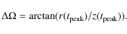
These two quantities are plotted in Figs. A.1 and A.2, respectively, as a function of
![\begin{figure}
\par\includegraphics[angle=90,width=18cm,clip]{12977f24.ps}
\end{figure}](/articles/aa/full_html/2010/05/aa12977-09/img169.png)
|
Figure A.11:
Same as Fig. A.9, but with
|
| Open with DEXTER | |
The radial displacement
![]() (Fig. A.1) is highly dependent on the pre-shock density since
its value depends on the cooling distance. However, the maximum
value is generally smaller than the pixel size used in the
models displayed in this paper. The effect of using
the z-axis approximation is thus insignificant. The biggest effect is found in
the right hand side of Fig. 2 in the model with
(Fig. A.1) is highly dependent on the pre-shock density since
its value depends on the cooling distance. However, the maximum
value is generally smaller than the pixel size used in the
models displayed in this paper. The effect of using
the z-axis approximation is thus insignificant. The biggest effect is found in
the right hand side of Fig. 2 in the model with
![]() cm-3. The pixel size is here 41.5 AU, which means that by using
the z-axis approximation we misplace the peak H2 emissivity 4 pixels in the
r-direction. Even in this case, however, the distortion introduced in the map morphology
is very small, because the angular displacement from the vertical,
cm-3. The pixel size is here 41.5 AU, which means that by using
the z-axis approximation we misplace the peak H2 emissivity 4 pixels in the
r-direction. Even in this case, however, the distortion introduced in the map morphology
is very small, because the angular displacement from the vertical,
![]() (Fig. A.2) remains low at <
(Fig. A.2) remains low at <![]() all along the bow shock, for all values
of preshock densities.
all along the bow shock, for all values
of preshock densities.
The effect of a lower
![]() on
on
![]() and
and
![]() is illustrated in Figs. A.3 and A.4 respectively,
in the case
is illustrated in Figs. A.3 and A.4 respectively,
in the case
![]() cm-3. Since the value of the radial displacement
depends on the distance travelled by the post-shock gas, it decreases in shocks
with a lower
cm-3. Since the value of the radial displacement
depends on the distance travelled by the post-shock gas, it decreases in shocks
with a lower
![]() ,
where the cooling distance is shorter. At the same time,
the distortion angle
,
where the cooling distance is shorter. At the same time,
the distortion angle
![]() of the peak emission region from the vertical
is virtually unchanged and remains small
of the peak emission region from the vertical
is virtually unchanged and remains small ![]()
![]() for
for
![]() .
In the case where
.
In the case where
![]() ,
the shock becomes J-type when
,
the shock becomes J-type when
![]() km s-1 due to H2 dissociation. The
bulk of rovibrational H2 emission is then emitted at much lower velocities
and higher compression than in C-shocks, and the angular deviation increases
dramatically to
km s-1 due to H2 dissociation. The
bulk of rovibrational H2 emission is then emitted at much lower velocities
and higher compression than in C-shocks, and the angular deviation increases
dramatically to
![]() .
However at the same time the cooling distance also
shrinks
dramatically, so that the offset from the vertical is completely negligible.
.
However at the same time the cooling distance also
shrinks
dramatically, so that the offset from the vertical is completely negligible.
We conclude that the z-axis approximation does not introduce a significant distortion of the bow emission morphology for the parameter range and map resolution explored in this paper.
| Figure A.12:
Same as Fig. A.9, but with
|
|
| Open with DEXTER | |
A.2 Stretching along the z-axis
In building our 3D model, we also assumed that the position along the z-axis
streamline is stretched uniformly to reach a full cooling distance of
![]() ,
where
,
where
![]() and
and
![]() are the distance travelled by the
post-shock gas at time
are the distance travelled by the
post-shock gas at time
![]() (where T =1000 K) perpendicular and
parallel to the shock surface, respectively. The rationale behind is that the
local velocity gradient dVz(t)/dz remains unchanged from the 1D case,
consistent with our use of the 1D temperature and emissivity distribution.
(where T =1000 K) perpendicular and
parallel to the shock surface, respectively. The rationale behind is that the
local velocity gradient dVz(t)/dz remains unchanged from the 1D case,
consistent with our use of the 1D temperature and emissivity distribution.
In other words, we use the following expression for the
approximate position of the post-shock gas along the z-axis:
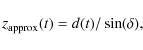
|
(A.9) |
where the ``stretching factor''
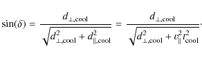
|
(A.10) |
In order to estimate the accuracy of this approximation we look at the exact position z(t) of the peak H2 emissivity along the z-axis, given in Eq. (A.6), and calculate the relative error
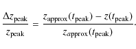
This quantity is displayed in (Fig. A.5) for various preshock densities and
The same graph in shown in (Fig. A.6) for lower values of
![]() and a pre-shock density
and a pre-shock density
![]() cm-3. The relative error on z tends to increase at lower b-field, but it does not exceed 35% in C-shocks. This is a rather high value but
corresponds to <3 pixels in our standard model. Furthermore, as with
cm-3. The relative error on z tends to increase at lower b-field, but it does not exceed 35% in C-shocks. This is a rather high value but
corresponds to <3 pixels in our standard model. Furthermore, as with
![]() ,
the absolute error
,
the absolute error
![]() in AUs actually decreases at lower b and would not be resolvable with current instruments (this is even more true for the J-shocks).
Therefore this approximation also seems acceptable for our range of
parameters.
in AUs actually decreases at lower b and would not be resolvable with current instruments (this is even more true for the J-shocks).
Therefore this approximation also seems acceptable for our range of
parameters.
A.3 Minimum scale of curvature
When using the output of 1D shock models, we are ignoring the
effect of the bow geometry on the velocity, density, and temperature of
the post-shock emitting material. Several effects will be present:
first, since the streamline is not exactly vertical, the emitting
material is moving in cones rather than cylinders and thus will suffer
some adiabatic expansion. However we have seen that the angle is very
small in the region of rovibrational H2 emission
(a few degrees, see Figs. A.2 and A.4)
therefore this effect can be neglected. Second, the bow curvature makes
the shock speed and postshock pressure vary along the shock surface,
introducing a transverse thermal and magnetic pressure gradient
across streamlines. Calculating such a complex effect is outside the
scope of the present paper. However we expect that it would remain
small with respect to 1D shock compression
if the local radius of curvature of the bow (determining these
transverse gradients)
is much larger than the characteristic scale of velocity (i.e.
pressure) variation in the H2 emission zone of the 1D shock, given by
|
(A.12) |
where
This characteristic scale is plotted along a bow of speed 40 km s-1 for various preshock densities in Fig. A.7, and for various
![]() in Fig. A.8.
Like the cooling distance, the scale varies almost inversely with
in Fig. A.8.
Like the cooling distance, the scale varies almost inversely with ![]() ,
dropping from 3000 AU to 60 AU for
,
dropping from 3000 AU to 60 AU for
![]() cm-3 when
cm-3 when
![]() ,
and decreasing in
proportion to
,
and decreasing in
proportion to
![]() for a fixed density (when the shock is C-type).
All the bowshock models presented in this paper (in particular those fitted to the OMC1 bowshock) have values of r0 that exceed this characteristic scale for the relevant
for a fixed density (when the shock is C-type).
All the bowshock models presented in this paper (in particular those fitted to the OMC1 bowshock) have values of r0 that exceed this characteristic scale for the relevant ![]() ,
suggesting that
the 1D approximation may be approximately valid, especially in the bow wings.
,
suggesting that
the 1D approximation may be approximately valid, especially in the bow wings.
Appendix B: Effect of magnetic field direction and viewing angle
Here we show in detail how the magnetic field direction and the
inclination to the line of sight affect the morphology of the projected
emission of our standard bow shock model.
The standard model has the following input parameters:
![]() cm3,
cm3,
![]() km s-1, b=5,
km s-1, b=5,
![]() ,
r0 = 1000 AU.
Figure A.9 displays the effect of changing the ``rotation'' angle
,
r0 = 1000 AU.
Figure A.9 displays the effect of changing the ``rotation'' angle
![]() from
from ![]() to
to ![]() (left to right)
and the inclination i from 0 to
(left to right)
and the inclination i from 0 to ![]() (top to bottom) when
(top to bottom) when
![]() (magnetic field perpendicular to the bow axis). Figure A.10 shows the
same for
(magnetic field perpendicular to the bow axis). Figure A.10 shows the
same for
![]() and Fig. A.11 the same for
and Fig. A.11 the same for
![]() .
The case of
.
The case of
![]() is illustrated in Fig. A.12, which contains a single column since
the result does not depend on
is illustrated in Fig. A.12, which contains a single column since
the result does not depend on ![]() (magnetic field parallel to the bow axis).
Note that maps for
(magnetic field parallel to the bow axis).
Note that maps for
![]() can be deduced
from the map with
can be deduced
from the map with
![]() by
applying mirror symmetry with respect to x=0. Similarly, maps for
by
applying mirror symmetry with respect to x=0. Similarly, maps for
![]() can be deduced
from the map with
can be deduced
from the map with
![]() ).
).
References
- Allen, D. A., & Burton, M. G. 1993, Nature, 363, 54 [NASA ADS] [CrossRef] [Google Scholar]
- Axon, D. J., & Taylor, K. 1984, MNRAS, 207, 241 [NASA ADS] [CrossRef] [Google Scholar]
- Baek, C. H., Kim, J., & Choi, M. 2009, ApJ, 690, 944 [NASA ADS] [CrossRef] [Google Scholar]
- Chrysostomou, A., Hough, J. H., Burton, M. G., & Tamura, M. 1994, MNRAS, 268, 325 [NASA ADS] [Google Scholar]
- Colgan, S. W. J., Schultz, A. S. B., Kaufman, M. J., Erickson, E. F., & Hollenbach, D. J. 2007, ApJ, 671, 536 [NASA ADS] [CrossRef] [Google Scholar]
- Crutcher, R. M., Troland, T. H., Lazareff, B., Paubert, G., & Kazès, I. 1999, ApJ, 514, L121 [NASA ADS] [CrossRef] [Google Scholar]
- Cunningham, N. 2006, Ph.D. Thesis, University of Colorado [Google Scholar]
- Davis, C. J., Froebrich, D., Stanke, T., et al. 2009, A&A, 496, 153 [NASA ADS] [CrossRef] [EDP Sciences] [Google Scholar]
- Draine, B. T. 1980, ApJ, 241, 1021 [NASA ADS] [CrossRef] [Google Scholar]
- Draine, B. T., & McKee, C. F. 1993, ARA&A, 31, 373 [NASA ADS] [CrossRef] [Google Scholar]
- Eislöffel, J., Mundt, R., & Bohm, K.-H. 1994, AJ, 108, 1042 [NASA ADS] [CrossRef] [Google Scholar]
- Flower, D. R., & Pineau des Forêts, G. 2003, MNRAS, 343, 390 [NASA ADS] [CrossRef] [Google Scholar]
- Genzel, R., Reid, M. J., Moran, J. M., & Downes, D. 1981, ApJ, 244, 884 [NASA ADS] [CrossRef] [Google Scholar]
- Greenhill, L. J., Gwinn, C. R., Schwartz, C., Moran, J. M., & Diamond, P. J. 1998, Nature, 396, 650 [NASA ADS] [CrossRef] [PubMed] [Google Scholar]
- Gustafsson, M. 2006, Ph.D. Thesis, University of Aarhus [Google Scholar]
- Gustafsson, M., Kristensen, L. E., Clénet, Y., et al. 2003, A&A, 411, 437 [NASA ADS] [CrossRef] [EDP Sciences] [Google Scholar]
- Hough, J. H., Axon, D. J., Burton, M. G., et al. 1986, MNRAS, 222, 629 [NASA ADS] [Google Scholar]
- Kristensen, L. E., Ravkilde, T. L., Field, D., Lemaire, J. L., & Pineau Des Forêts, G. 2007, A&A, 469, 561 [NASA ADS] [CrossRef] [EDP Sciences] [Google Scholar]
- Kristensen, L. E., Ravkilde, T. L., Pineau Des Forêts, G., et al. 2008, A&A, 477, 203 [NASA ADS] [CrossRef] [EDP Sciences] [Google Scholar]
- Lacombe, F., Gendron, E., Rouan, D., et al. 2004, A&A, 417, L5 [NASA ADS] [CrossRef] [EDP Sciences] [Google Scholar]
- Le Bourlot, J., Pineau des Forêts, G., Flower, D. R., & Cabrit, S. 2002, MNRAS, 332, 985 [NASA ADS] [CrossRef] [Google Scholar]
- Menten, K. M., Reid, M. J., Forbrich, J., & Brunthaler, A. 2007, A&A, 474, 515 [NASA ADS] [CrossRef] [EDP Sciences] [Google Scholar]
- Nissen, H. D., Gustafsson, M., Lemaire, J. L., et al. 2007, A&A, 466, 949 [NASA ADS] [CrossRef] [EDP Sciences] [Google Scholar]
- Norris, R. P. 1984, MNRAS, 207, 127 [NASA ADS] [Google Scholar]
- O'Connell, B., Smith, M. D., Davis, C. J., et al. 2004, A&A, 419, 975 [NASA ADS] [CrossRef] [EDP Sciences] [Google Scholar]
- O'Connell, B., Smith, M. D., Froebrich, D., Davis, C. J., & Eislöffel, J. 2005, A&A, 431, 223 [NASA ADS] [CrossRef] [EDP Sciences] [Google Scholar]
- Raga, A. C., de Gouveia Dal Pino, E. M., Noriega-Crespo, A., Mininni, P. D., & Velázquez, P. F. 2002, A&A, 392, 267 [NASA ADS] [CrossRef] [EDP Sciences] [Google Scholar]
- Raga, A. C., Esquivel, A., Riera, A., & Velázquez, P. F. 2007, ApJ, 668, 310 [NASA ADS] [CrossRef] [Google Scholar]
- Ravkilde, T. L. 2007, Master's thesis, Department of Physics and Astronomy, University of Aarhus, Ny Munkegade, Bld. 1520, DK-8000 Aarhus C, Denmark, available online at http://www.phys.au.dk/ ravkilde/msc/ [Google Scholar]
- Reipurth, B., & Bally, J. 2001, ARA&A, 39, 403 [NASA ADS] [CrossRef] [Google Scholar]
- Schultz, A. S. B., Colgan, S. W. J., Erickson, E. F., et al. 1999, ApJ, 511, 282 [NASA ADS] [CrossRef] [Google Scholar]
- Simpson, J. P., Colgan, S. W. J., Erickson, E. F., Burton, M. G., & Schultz, A. S. B. 2006, ApJ, 642, 339 [NASA ADS] [CrossRef] [Google Scholar]
- Smith, M. D. 1991, MNRAS, 252, 378 [NASA ADS] [Google Scholar]
- Smith, M. D. 1992, ApJ, 390, 447 [NASA ADS] [CrossRef] [Google Scholar]
- Smith, M. D., Khanzadyan, T., & Davis, C. J. 2003, MNRAS, 339, 524 [NASA ADS] [CrossRef] [Google Scholar]
- Smith, M. D., O'Connell, B., & Davis, C. J. 2007, A&A, 466, 565 [NASA ADS] [CrossRef] [EDP Sciences] [Google Scholar]
- Stolovy, S. R., Burton, M. G., Erickson, E. F., et al. 1998, ApJ, 492, L151 [NASA ADS] [CrossRef] [Google Scholar]
- Suttner, G., Smith, M. D., Yorke, H. W., & Zinnecker, H. 1997, A&A, 318, 595 [NASA ADS] [Google Scholar]
- Takami, M., Chrysostomou, A., Ray, T. P., et al. 2006, ApJ, 641, 357 [NASA ADS] [CrossRef] [Google Scholar]
- Takami, M., Beck, T. L., Pyo, T.-S., McGregor, P., & Davis, C. 2007, ApJ, 670, L33 [NASA ADS] [CrossRef] [Google Scholar]
- Tamura, M., Kandori, R., Kusakabe, N., et al. 2006, ApJ, 649, L29 [NASA ADS] [CrossRef] [Google Scholar]
Footnotes
- ... C-shocks
![[*]](/icons/foot_motif.png)
- In our standard model the emission from J-shock regions is orders of magnitude weaker than the emission from the surrounding C-shocks. However, the relative strength of the emission in J- and C-shocks is dependent on the pre-shock density, the b-value, and the bow velocity (Kristensen et al. 2009, in prep.). Thus, bow shocks exist for which the brightness from the J-shocks is comparable to that of the C-shocks. That is, dissociative regions in a bow shock do not always produce a large decrease in H2emission.
All Tables
Table 1: Model parameters of the model that best reproduces the observations.
All Figures
| |
Figure 1:
Geometry of the bow shock model. The bow shock is moving along
the z-axis at an angle, i, to the line of sight which lies in the
z-y plane. The direction of a
uniform magnetic field is specified by the angles |
| Open with DEXTER | |
| In the text | |
|
|
Figure 2:
Brightness in Wm-2 sr-1, size and thickness in AU
of a series of shocks as a
function of pre-shock
density.
From top to bottom, the pre-shock density is
106, 105, 104 cm-3.
The shock is seen edge-on,
|
| Open with DEXTER | |
| In the text | |
|
|
Figure 3:
Brightness, size and morphology as a function of bow velocity. From
top to bottom the velocity is 60, 50, 40, and 30 km s-1. The shock is seen edge-on,
|
| Open with DEXTER | |
| In the text | |
|
|
Figure 4:
Brightness and thickness as a function of the magnetic field scaling
factor, b. From top to bottom, b = 8, 5, and 1. The shock is seen edge-on,
|
| Open with DEXTER | |
| In the text | |
|
|
Figure 5:
Left: morphology change as a function of the magnetic
field direction |
| Open with DEXTER | |
| In the text | |
|
|
Figure 6:
Morphology change as a function of the magnetic field direction
angle |
| Open with DEXTER | |
| In the text | |
|
|
Figure 7:
Morphology change as a function of the inclination angle, i. From
top to bottom,
|
| Open with DEXTER | |
| In the text | |
|
|
Figure 8:
Example of an excitation diagram from the 3D model in a region where the
gas is not completely thermalized. The v=1-0 band and the v=2-1
band do not line up. Both bands are well fitted individual by the same
excitation temperature of 2600 K (dotted and dashed line,
respectively), but with an offset. If both bands are included in the
fit (full line), the resulting excitation temperature
of 1900 K is lower than if only one band is used. The input
parameters of the model are
|
| Open with DEXTER | |
| In the text | |
|
|
Figure 9:
Excitation temperature as a function of the magnetic field
direction |
| Open with DEXTER | |
| In the text | |
|
|
Figure 10:
Centroid radial velocities as a function of inclination and
magnetic field direction. From top to bottom
|
| Open with DEXTER | |
| In the text | |
|
|
Figure 11:
Deviations in column density of H2 levels of the 3D model with
respect to the 1D shock in the apex. The column densities of the
emission peak in the 3D model (+ -signs) are higher than those of the
1D apex shock, whereas the average column density of the 3D model is
lower (diamonds). The column densities of the emission peak deviate more
from the 1D shock, both in terms of absolute values and in the
difference between the v=1 and the v=2 levels, than the average column
density of the 3D model. The model parameters are
|
| Open with DEXTER | |
| In the text | |
|
|
Figure 12:
Brightness of a bow shock in OMC1 observed
at ESO-VLT and the corresponding radial velocity map from
Nissen et al. (2007) ( upper row) compared to the best fit 3D model ( lower row). The
observational data has been rotated clockwise by 55 |
| Open with DEXTER | |
| In the text | |
|
|
Figure 13: Contours of brightness and radial velocity from the observations (blue) and the model (red). The contour levels in the three brightness plots are 0.2, 0.5, and 0.8 times the maximum brigthness. In the plot of radial velocity the contours delineate -20, -15, -10, -5, and 0 km s-1. |
| Open with DEXTER | |
| In the text | |
|
|
Figure A.1:
The radial displacement (see Eq. (A.7)) of the peak v=1-0 S(1) H2 emissivity
from the z-axis, for planar shocks along a bow with
|
| Open with DEXTER | |
| In the text | |
|
|
Figure A.2: The angular displacement in degrees (see Eq. (A.8)) of the peak v=1-0 S(1) H2 emissivity from the z-direction, for the same models as in Fig. A.1. |
| Open with DEXTER | |
| In the text | |
|
|
Figure A.3:
The radial displacement (see Eq. (A.7)) of the peak v=1-0 S(1) H2 emissivity
from the z-axis, for planar shocks along a bow with
|
| Open with DEXTER | |
| In the text | |
|
|
Figure A.4: The angular displacement in degrees (see Eq. (A.8)) of the peak v=1-0 S(1) H2 emissivity from the z-direction, for the same models as in Fig. A.3. |
| Open with DEXTER | |
| In the text | |
|
|
Figure A.5: The relative error in the z-position (see Eq. (A.11)) of the peak v=1-0 S(1) H2 emissivity for the same models as in Fig. A.1. |
| Open with DEXTER | |
| In the text | |
|
|
Figure A.6: The relative error in the z-position (see Eq. (A.11)) of the peak v=1-0 S(1) H2 emissivity for the same models as in Fig. A.3. |
| Open with DEXTER | |
| In the text | |
|
|
Figure A.7:
Characteristic 1D velocity variation scale
for planar models with
|
| Open with DEXTER | |
| In the text | |
|
|
Figure A.8:
Characteristic 1D velocity variation scale for planar
models with
|
| Open with DEXTER | |
| In the text | |
|
|
Figure A.9:
The standard shock with
|
| Open with DEXTER | |
| In the text | |
|
|
Figure A.10:
Same as Fig. A.9, but with
|
| Open with DEXTER | |
| In the text | |
|
|
Figure A.11:
Same as Fig. A.9, but with
|
| Open with DEXTER | |
| In the text | |
| |
Figure A.12:
Same as Fig. A.9, but with
|
| Open with DEXTER | |
| In the text | |
Copyright ESO 2010
Current usage metrics show cumulative count of Article Views (full-text article views including HTML views, PDF and ePub downloads, according to the available data) and Abstracts Views on Vision4Press platform.
Data correspond to usage on the plateform after 2015. The current usage metrics is available 48-96 hours after online publication and is updated daily on week days.
Initial download of the metrics may take a while.