| Issue |
A&A
Volume 510, February 2010
|
|
|---|---|---|
| Article Number | A38 | |
| Number of page(s) | 12 | |
| Section | Cosmology (including clusters of galaxies) | |
| DOI | https://doi.org/10.1051/0004-6361/200912823 | |
| Published online | 04 February 2010 | |
Filaments in observed and mock galaxy catalogues
R. S. Stoica1 - V. J. Martínez2 - E. Saar3
1 - Université Lille 1, Laboratoire Paul Painlevé,
59655 Villeneuve d'Ascq Cedex, France
2 - Observatori Astronòmic and Departament d'Astronomia i Astrofísica,
Universitat de València, Apartat de correus 22085, 46071 València,
Spain
3 - Tartu Observatoorium, Tõravere 61602, Estonia
Received 3 July 2009 / Accepted 10 November 2009
Abstract
Context. The main feature of the spatial large-scale
galaxy distribution is an intricate network of galaxy filaments.
Although many attempts have been made to quantify this network, there
is no unique and satisfactory recipe for that yet.
Aims. The present paper compares the filaments in
the real data and in the numerical models, to see if our best models
reproduce statistically the filamentary network of galaxies.
Methods. We apply an object point process with
interactions (the Bisous process) to trace and describe the filamentary
network both in the observed samples (the R2dFGRS catalogue) and in the
numerical models that have been prepared to mimic the data. We compare
the networks.
Results. We find that the properties of filaments in
numerical models (mock samples) have a large variance. A few mock
samples display filaments that resemble the observed filaments, but
usually the model filaments are much shorter and do not form an
extended network.
Conclusions. We conclude that although we can build
numerical models that are similar to observations in many respects,
they may fail yet to explain the filamentary structure seen in the
data. The Bisous-built filaments are a good test for such a structure.
Key words: cosmology: large-scale structure of Universe - methods: data analysis - methods: statistical
1 Introduction
The large-scale structure of the Universe traced by the
three-dimensional distribution of galaxies shows intriguing patterns:
filamentary structures connecting huge clusters surround nearly empty
regions, the so-called voids. As an example, we show here a map from
the 2dF Galaxy Redshift Survey (R2dFGRS, Colless
et al. 2001). As an illustration
of the filamentary network, Fig. 1 shows
the positions of galaxies in two ![]() thick slices from two
spatial regions that the R2dFGRS covered. Distances are given in
redshifts z.
thick slices from two
spatial regions that the R2dFGRS covered. Distances are given in
redshifts z.
![\begin{figure}
\par\includegraphics[width=14cm,clip]{12823fg1.eps}
\end{figure}](/articles/aa/full_html/2010/02/aa12823-09/img7.png)
|
Figure 1:
Galaxy map for two R2dFGRS slices of the
thickness of |
| Open with DEXTER | |
Filaments visually dominate the galaxy maps. Real three-dimensional filaments have been extracted from the galaxy distribution as a result of special observational projects (Pimbblet & Drinkwater 2004), or by searching for filaments in the R2dFGRS catalogue (Pimbblet et al. 2004). These filaments have been searched for between galaxy clusters, determining the density distribution and deciding if it is filamentary, individually for every filament (Pimbblet 2005). Filaments are also suspected to hide half of the warm gas in the Universe; an example of a discovery of such gas is the paper by Werner et al. (2008).
However, there are still no standard methods to describe the observed filamentary structure, but much work is being done in this direction. The usual second-order summary statistics as the two-point correlation function or the power spectrum do not provide morphological information. Minkowski functionals, minimal spanning tree (MST), percolation and shapefinders have been introduced for this purpose (for a review see Martínez & Saar 2002).
The minimal spanning tree was introduced in cosmology by Barrow et al. (1985). It is a unique graph that connects all points of the process without closed loops, but it describes mainly the local nearest-neighbour distribution and does not give us the global and large-scale properties of the filamentary network. A recent development of these ideas is presented by Colberg (2007). He applies a minimal spanning tree on a grid, and works close to the percolation regime - this allows the study of the global structure of the galaxy distribution. We note that using a grid introduces a smoothed density, and this is typical for other recent approaches, too.
In order to describe the filamentary structure of continuous density fields, a skeleton method has been proposed and developed by Eriksen et al. (2004) and Novikov et al. (2006). The skeleton is determined by segments parallel to the gradient of the field, connecting saddle points to local maxima. Calculating the skeleton involves interpolation and smoothing the point distribution, which introduces an extra parameter, which is the band-width of the kernel function used to estimate the density field from the point distribution, typically a Gaussian function. This is generally the case for most of the density-based approaches. The skeleton method was first applied for two-dimensional maps, an approach to study the cosmic microwave sky background (Eriksen et al. 2004). The method was adapted for 3-D maps (Sousbie et al. 2008a) and was applied to the Sloan Digital Sky Survey by Sousbie et al. (2008b), providing by means of the length of the skeleton, a good distinguishing tool for the analysis of the filamentary structures. The formalism has recently been further developed and applied to study the evolution of filamentary structure in simulations (Sousbie et al. 2009).
Another approach is that of Aragón-Calvo et al. (2007a) (see also Aragón-Calvo 2007). They use the Delaunay Triangulation Field Estimator (DFTE) to reconstruct the density field for the galaxy distribution, and apply the Multiscale Morphology Filter (MMF) to identify various structures, as for instance clusters, walls, filaments and voids (Aragón-Calvo et al. 2007b). As a further development, this group has used the watershed algorithm to describe the global properties of the density field (Aragon-Calvo et al. 2008).
A new direction is to use the second-order properties (the Hessian matrix) of the density field (Bond et al. 2009) or the deformation tensor (Forero-Romero et al. 2008). As is shown in these papers, this allows them to trace and classify different features of the fields.
Our approach does not introduce the density estimation step; we consider the galaxy distribution as a marked point process. In an earlier paper (Stoica et al. 2005b), we proposed to use an automated method to trace filaments for realisations of marked point processes, which has been shown to work well for the detection of road networks in remote sensing situations (Stoica et al. 2004,2002; Lacoste et al. 2005). This method is based on the Candy model, a marked point process where segments serve as marks. The Candy model can be applied to 2-D filaments, and we tested it on simulated galaxy distributions. The filaments we found delineated well the filaments detected by eye.
Based on our previous experience with the Candy model, we generalised the approach for three dimensions. As the interactions between the structure elements are more complex in three dimensions, we had to define a more complex model, the Bisous model (Stoica et al. 2005a). This model gives a general framework for the construction of complex patterns made of simple interacting objects. In our case, it can be seen as a generalisation of the Candy model. We applied the Bisous model to trace and describe the filaments in the R2dFGRS (Stoica et al. 2007b) and demonstrated that it works well.
In the paper cited above we chose the observational samples from the main magnitude-limited R2dFGRS catalogue, selecting the spatial regions to have approximately constant spatial densities. But a strict application of the Bisous process demands a truly constant spatial density (intensity). In this paper, we will apply the Bisous process to compare the observational data with mock catalogues, specially built to represent the R2dFGRS survey. To obtain strict statistical test results, we use here volume-limited subsamples of the R2dFGRS and of the mock catalogues. We trace the filamentary network in all our catalogues and compare its properties.
2 Mathematical tools
In this section we describe the main tools we use to study the large-scale filaments. The key idea is to see this filamentary structure as a realisation of a marked point process. Under this hypothesis, the cosmic web can be considered as a random configuration of segments or thin cylinders that interact, forming a network of filaments. Hence, the morphological and quantitative characteristics of these complex geometrical objects can be obtained by following a straightforward procedure: constructing a model, sampling the probability density describing the model, and, finally, applying the methods of statistical inference.
We have given a more detailed description of these methods in a previous paper (Stoica et al. 2007b).
2.1 Marked point processes
A popular model for the spatial distribution of galaxies is a point
process on K (a compact subset of
![]() ,
the cosmologist's sample
volume), a random configuration of points
,
the cosmologist's sample
volume), a random configuration of points
![]() ,
lying in K. Let
,
lying in K. Let ![]() be the volume of K.
be the volume of K.
We may associate characteristics or marks to the points. For
instance,
to each point in a configuration ![]() ,
shape parameters describing
simple geometrical objects may be attached. Let
,
shape parameters describing
simple geometrical objects may be attached. Let
![]() be
the probability measure space defining these marks. A marked or object
point process on
be
the probability measure space defining these marks. A marked or object
point process on ![]() is the random configuration
is the random configuration
![]() ,
with
,
with ![]() for all
for all ![]() in a way that the
locations process is a point process on K. For our
purposes, the
point process is considered finite and simple, i.e. the number
of points in a configuration is finite and
in a way that the
locations process is a point process on K. For our
purposes, the
point process is considered finite and simple, i.e. the number
of points in a configuration is finite and
![]() ,
for any
i,j so that
,
for any
i,j so that
![]() .
.
In case of the simplest marked point process, the objects do
not
interact. The Poisson object point process is the most appropriate
choice for such a situation. This process chooses a number of objects
according to a Poisson law of the intensity parameter ![]() ,
gives
a random independent location to each object uniformly in K
and a
random shape or mark chosen independently according to
,
gives
a random independent location to each object uniformly in K
and a
random shape or mark chosen independently according to ![]() .
The
Poisson object point process has the great advantage that it can be
described by analytical formulae. Still, it is too simple whenever
the interactions of objects are to be taken into account.
.
The
Poisson object point process has the great advantage that it can be
described by analytical formulae. Still, it is too simple whenever
the interactions of objects are to be taken into account.
The solution to the latter problem is to specify a probability
density
![]() that takes into account
interactions between the
objects. This probability density is specified with respect to the
reference measure given by the Poisson object point process. There is
a lot of freedom in building such densities, provided that they are
integrable with respect to the reference measure and are locally
stable. This second condition requires that there exists
that takes into account
interactions between the
objects. This probability density is specified with respect to the
reference measure given by the Poisson object point process. There is
a lot of freedom in building such densities, provided that they are
integrable with respect to the reference measure and are locally
stable. This second condition requires that there exists
![]() so that
so that
![]() for
any
for
any ![]() .
Local stability implies integrability. It is also an
important condition, guaranteeing that the simulation algorithms for
sampling such models have good convergence properties.
.
Local stability implies integrability. It is also an
important condition, guaranteeing that the simulation algorithms for
sampling such models have good convergence properties.
For further reading and a comprehensive mathematical presentation of object point processes, we recommend the monographs by van Lieshout (2000), Møller & Waagepetersen (2003), Stoyan et al. (1995), and Illian et al. (2008).
2.2 Bisous model
In this section, we shall describe the probability density of the Bisous model for the network of cosmic filaments. The Bisous model is a marked point process that was designed to generate and analyse random spatial patterns (Stoica et al. 2005a,2007b).Random spatial patterns are complex geometrical structures composed of
rather simple objects that interact. We can describe our problem as
follows: in a region K of a finite volume, we
observe a finite
number of galaxies
![]() .
The positions of
these galaxies form a complicated filamentary network. Modelling it by
a network of thin cylinders that can get connected and aligned in a
certain way, a marked point process - the Bisous model - can be
built in order to describe it.
.
The positions of
these galaxies form a complicated filamentary network. Modelling it by
a network of thin cylinders that can get connected and aligned in a
certain way, a marked point process - the Bisous model - can be
built in order to describe it.
A random cylinder is an object characterised by its centre k
and its
mark giving the shape parameters. The shape parameters of a cylinder
are the radius r, the height h
and the orientation vector
![]() .
We consider the radius and height parameters as fixed,
whereas the orientation vector parameters
.
We consider the radius and height parameters as fixed,
whereas the orientation vector parameters
![]() are
uniformly distributed on
are
uniformly distributed on
![]() so
that
so
that
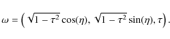
|
(1) |
For our purposes, throughout this paper the shape of a cylinder is denoted by
A cylinder ![]() has q=2 extremity rigid points. We centre
around each of these points a sphere of the radius
has q=2 extremity rigid points. We centre
around each of these points a sphere of the radius ![]() .
These two
spheres form an attraction region that plays an important role in
defining connectivity and alignment rules for cylinders. We illustrate
the basic cylinder in Fig. 2, where it is
centred at the
coordinate origin and its symmetry axis is parallel to Ox.
The
coordinates of the extremity points are
.
These two
spheres form an attraction region that plays an important role in
defining connectivity and alignment rules for cylinders. We illustrate
the basic cylinder in Fig. 2, where it is
centred at the
coordinate origin and its symmetry axis is parallel to Ox.
The
coordinates of the extremity points are
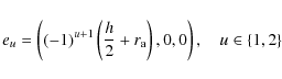
|
(2) |
and the orientation vector is
![\begin{figure}
\par\includegraphics[width=7cm,clip]{12823fg2.eps}
\end{figure}](/articles/aa/full_html/2010/02/aa12823-09/img37.png)
|
Figure 2: A thin cylinder that generates the filamentary network. |
| Open with DEXTER | |
The probability density for a marked point process based on random
cylinders can be written using the Gibbs modelling framework:
![\begin{displaymath}p({\vec y}\vert \theta) = \frac{\exp\left[-U({\vec y}\vert\theta)\right]}{\alpha}
\end{displaymath}](/articles/aa/full_html/2010/02/aa12823-09/img38.png)
where
Modelling the filamentary network induced by the galaxy positions needs two assumptions. The first assumption is that locally, galaxies may be grouped together inside a rather small thin cylinder. The second assumption is that such small cylinders may combine to extend a filament if neighbouring cylinders are aligned in similar directions.
Following these two ideas the energy function given
by (3)
can be specified as:
where
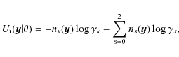
2.3 Data energy
The data energy of a configuration of cylinders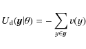
where
The cylinder potential is built taking into account local
criteria
such as the density, spread and number of galaxies. To formulate these
criteria, an extra cylinder is attached to each cylinder y,
with
exactly the same parameters as y, except for the
radius which equals 2r. Let
![]() be
the shadow of s(y) obtained
by the
subtraction of the initial cylinder from the extra cylinder, as shown
in Fig. 3.
Then, each cylinder y is divided in
three equal volumes along its main symmetry axis, and we denote by
s1(y), s2(y)
and s3(y)
their corresponding shapes.
be
the shadow of s(y) obtained
by the
subtraction of the initial cylinder from the extra cylinder, as shown
in Fig. 3.
Then, each cylinder y is divided in
three equal volumes along its main symmetry axis, and we denote by
s1(y), s2(y)
and s3(y)
their corresponding shapes.
![\begin{figure}
\par\includegraphics[width=6.1cm,clip]{12823fg3.eps}
\end{figure}](/articles/aa/full_html/2010/02/aa12823-09/img49.png)
|
Figure 3: Two-dimensional projection of a thin cylinder with its shadow within a pattern of galaxies. |
| Open with DEXTER | |
The local density condition verifies that the density of galaxies
inside s(y) is higher than the
density of galaxies in
![]() ,
and it can be expressed as follows:
,
and it can be expressed as follows:
| (6) |
where
The even location of the galaxies along the cylinder main axis
is ensured by the spread condition,
which is formulated as
|
(7) |
where
If both these conditions are fulfilled, then v(y)
is given by the
difference between the number of galaxies contained in the cylinder and
the number of galaxies contained in its shadow:
| (8) |
Whenever any of the previous conditions is violated, a positive value
A segment which does not fulfill the required conditions can
still be
integrated into the network by the parameter ![]() .
This should result in more complete networks and better mixing
properties to the method.
.
This should result in more complete networks and better mixing
properties to the method.
We note that we have chosen cylinders as the objects here in order to trace filaments in the galaxy distribution. Such objects are tools at our disposal and any object can be chosen; as an example, Stoica et al. (2005a) have built systems of flat elements (walls) and of regular polytopes (galaxy clusters), based on the Bisous process.
2.4 Interaction energy
The interaction energy takes into account the interactions between
cylinders. It is the model component ensuring that the cylinders form
a filamentary network, and it is given by
where
We define the interactions that allow the configuration of cylinders to trace the filamentary network below. To illustrate these definitions, we show an example configuration of cylinders (in two dimensions) in Fig. 4.
Two cylinders are considered repulsive, if they are rejecting
each
other and if they are not orthogonal. We declare that two cylinders
![]() and
and
![]() reject
each other if
their centres are closer than the cylinder height,
d(k1,k2)
<
h. Two cylinders are considered to be orthogonal if
reject
each other if
their centres are closer than the cylinder height,
d(k1,k2)
<
h. Two cylinders are considered to be orthogonal if
![]() ,
where
,
where ![]() is the scalar
product of the two orientation vectors and
is the scalar
product of the two orientation vectors and
![]() is
a predefined parameter. So, we allow a certain range of mutual angles
between cylinders that we consider orthogonal.
is
a predefined parameter. So, we allow a certain range of mutual angles
between cylinders that we consider orthogonal.
Two cylinders are connected if they attract each other, do not
reject each other and are well aligned. Two cylinders attract
each other if only one extremity point of the first cylinder is
contained in the attraction region of the other cylinder. The
cylinders are ``magnetised'' in the sense that they cannot attract
each other through extremity points having the same index. Two
cylinders are well aligned if
![]() ,
where
,
where ![]() is a predefined
parameter.
is a predefined
parameter.
Take now a look at Fig. 4. According to the previous definitions, we observe that the cylinders c1, c2 and c3 are connected. The cylinders c1 and c3 are connected to the network through one extremity point, while c2 is connected to the network through both extremity points. The cylinders c4 and c5 are not connected to anything - c4 is not well aligned with c2, the angle between their directions is too large, and c5 is not attracted to any other cylinder. It is important to notice that the cylinders c3 and c4 are not interacting - they are wrongly ``polarised'', their overlapping extremity points have the same index. The cylinder c5 is rejecting the cylinders c2 and c4(the centres of these cylinders are close), but as it is rather orthogonal both to c2 and c4, it is not repulsing them. The cylinders c2 and c4 reject each other and are not orthogonal, so they form a repulsive pair.
Altogether, the configuration at Fig. 4 adds to the interaction energy contributions from three connected cylinders (one doubly-connected, c2, and two single-connected, c1 and c3), and from one repulsive cylinder pair (c2-c4).
| Figure 4: Two-dimensional representation of interacting cylinders. |
|
| Open with DEXTER | |
The complete model (3)
that includes the definitions
of the data energy and of the interaction energy given
by (5)
and (9)
is well defined
for parameters as ![]() ,
,
![]() and
and
![]() .
The definitions of the interactions
and the parameter ranges chosen ensure that the complete model is
locally stable and Markov in the sense of
Ripley-Kelly (Stoica
et al. 2005a). For cosmologists it means that
we can safely use this model without expecting any dangers (numerical,
convergence, etc.).
.
The definitions of the interactions
and the parameter ranges chosen ensure that the complete model is
locally stable and Markov in the sense of
Ripley-Kelly (Stoica
et al. 2005a). For cosmologists it means that
we can safely use this model without expecting any dangers (numerical,
convergence, etc.).
2.5 Simulation
Several Monte Carlo techniques are available to simulate marked point processes: spatial birth-and-death processes, Metropolis-Hastings algorithms, reversible jump dynamics or more recent exact simulation techniques (Kendall & Møller 2000; Green 1995; Geyer & Møller 1994; Geyer 1999; van Lieshout & Stoica 2006; Preston 1977; van Lieshout 2000).In this paper, we need to sample from the joint probability density
law ![]() .
This is done by using an iterative Monte Carlo
algorithm. An iteration of the algorithm consists of two steps. First,
a value for the parameter
.
This is done by using an iterative Monte Carlo
algorithm. An iteration of the algorithm consists of two steps. First,
a value for the parameter ![]() is chosen with respect to
is chosen with respect to ![]() .
Then, conditionally on
.
Then, conditionally on ![]() ,
a cylinder pattern is
sampled from
,
a cylinder pattern is
sampled from ![]() using a Metropolis-Hastings
algorithm (Geyer
1999; Geyer
& Møller 1994).
using a Metropolis-Hastings
algorithm (Geyer
1999; Geyer
& Møller 1994).
The Metropolis-Hastings algorithm for sampling the conditional
law
![]() has a transition kernel based
on three types of
moves. The first move is called birth and proposes
to add a
new cylinder to the present configuration. This new cylinder can be
added uniformly in K or can be randomly connected
with the rest of
the network. This mechanism helps to build a connected network. The
second move is called death, and proposes to
eliminate a
randomly chosen cylinder. The role of this second move is to ensure
the detailed balance of the simulated Markov chain and its convergence
towards the equilibrium distribution. A third move can be added to
improve the mixing properties of the sampling algorithm. This
third move is called change; it randomly chooses a
cylinder in
the configuration and proposes to ``slightly'' change its parameters
using simple probability distributions. For specific details
concerning the implementation of this dynamics we
recommend Lieshout
& Stoica (2003) and Stoica
et al. (2005a).
has a transition kernel based
on three types of
moves. The first move is called birth and proposes
to add a
new cylinder to the present configuration. This new cylinder can be
added uniformly in K or can be randomly connected
with the rest of
the network. This mechanism helps to build a connected network. The
second move is called death, and proposes to
eliminate a
randomly chosen cylinder. The role of this second move is to ensure
the detailed balance of the simulated Markov chain and its convergence
towards the equilibrium distribution. A third move can be added to
improve the mixing properties of the sampling algorithm. This
third move is called change; it randomly chooses a
cylinder in
the configuration and proposes to ``slightly'' change its parameters
using simple probability distributions. For specific details
concerning the implementation of this dynamics we
recommend Lieshout
& Stoica (2003) and Stoica
et al. (2005a).
Whenever the maximisation of the joint law
![]() is
needed,
the previously described sampling mechanism can be integrated into a
simulated annealing algorithm. The simulated annealing algorithm is
built by sampling from
is
needed,
the previously described sampling mechanism can be integrated into a
simulated annealing algorithm. The simulated annealing algorithm is
built by sampling from
![]() ,
while T goes slowly to
zero. Stoica et al.
(2005a) proved the convergence of such simulated
annealing for simulating marked point processes, when a logarithmic
cooling schedule is used. According to this result, the temperature is
lowered as
,
while T goes slowly to
zero. Stoica et al.
(2005a) proved the convergence of such simulated
annealing for simulating marked point processes, when a logarithmic
cooling schedule is used. According to this result, the temperature is
lowered as

we use T0=10 for the initial temperature.
2.6 Statistical inference
One straightforward application of the simulation dynamics is the estimation of the filamentary structure in a field of galaxies together with the parameter estimates. These estimates are given by:
where
However, the solution we obtain is not unique. In practice,
the shape of the prior law ![]() may influence the solution,
making the result to look more random compared with a result obtained
for fixed values of parameters. Therefore, it is reasonable to wonder
how precise the estimate is, that is if an element of the pattern
really belongs to the pattern, or if its presence is due to random
effects (Stoica
et al. 2007a,b).
may influence the solution,
making the result to look more random compared with a result obtained
for fixed values of parameters. Therefore, it is reasonable to wonder
how precise the estimate is, that is if an element of the pattern
really belongs to the pattern, or if its presence is due to random
effects (Stoica
et al. 2007a,b).
For compact subregions
![]() ,
we can compute or give Monte Carlo approximations
for average quantities such as
,
we can compute or give Monte Carlo approximations
for average quantities such as
![\begin{displaymath}{\rm E}_{({\vec Y},\Theta)}\left[f({\cal R}, Z({\vec Y}))\right],
\end{displaymath}](/articles/aa/full_html/2010/02/aa12823-09/img85.png)
where E denotes the expectation value over the data and model parameter space, and
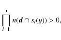
If
![]() (where
(where
![]() is the
indicator function), then the expression (12)
represents the probability of how often the considered model includes
or visits the region
is the
indicator function), then the expression (12)
represents the probability of how often the considered model includes
or visits the region ![]() .
Furthermore, if K is partitioned into a
finite collection of small disjoint cells
.
Furthermore, if K is partitioned into a
finite collection of small disjoint cells
![]() ,
then a visit probability map can be
obtained. This map is given by the partition together with the value
,
then a visit probability map can be
obtained. This map is given by the partition together with the value
![]() associated
to each cell. The map is defined by the model and by the
parameters of the simulation algorithm; its resolution is given by the
cell partition.
associated
to each cell. The map is defined by the model and by the
parameters of the simulation algorithm; its resolution is given by the
cell partition.
The sufficient statistics of the model (9) -
the interaction parameters ![]() and ns,
s=(0,1,2) -
describe the size of the filamentary network and quantify the
morphological properties of the network. Therefore, they are suitable
as a general characterisation of the filamentarity of a galaxy
catalogue. This renders the comparison of the networks of different
regions and/or
different catalogues perfectly possible. Here, we use the
sufficient statistics to characterise the real data and the mock
catalogues.
and ns,
s=(0,1,2) -
describe the size of the filamentary network and quantify the
morphological properties of the network. Therefore, they are suitable
as a general characterisation of the filamentarity of a galaxy
catalogue. This renders the comparison of the networks of different
regions and/or
different catalogues perfectly possible. Here, we use the
sufficient statistics to characterise the real data and the mock
catalogues.
The visit maps show the location and configuration of the filament network. Still, the detection of filaments and this verification test depend on the selected model. It is reasonable to ask if these results are obtained because the data exhibits a filamentary structure or just because of the way the model parameters are selected.
The sufficient statistics can be used to build a statistical test in order to answer the previous question. For a given data catalogue, samples of the model are obtained, so the means of the sufficient statistics can be then computed. The same operation, using exactly the same model parameters, can be repeated whenever an artificial point field - or a synthetic data catalogue - is used. If the artificial field is the realisation of a binomial point process having the same number of points as the number of galaxies in the original data set, the sufficient statistics are expected to have very low values - there is no global structure in a such binomial field. If the values of the sufficient statistics for these binomial fields were large, this would mean that the filamentary structure is due to the parameters, not to the data. Comparing the values obtained for the original data sets with Monte Carlo envelopes found for artificial point fields, we can compute Monte Carlo p-values to test the hypothesis of the existence of the filamentary structure in the original data catalogue (Stoica et al. 2007a,b).
3 Data
We apply our algorithms to a real data catalogue and compare the results with those obtained for 22 mock catalogues, specially generated to simulate all main features of the real data.
![\begin{figure}
\par\includegraphics[width=16.5cm,clip]{12823fg5.eps}
\end{figure}](/articles/aa/full_html/2010/02/aa12823-09/img93.png)
|
Figure 5: The geometry and coordinates of the data bricks. Right panel: all 2dF galaxies inside a large contiguous area of the northern wedge are shown in blue (up to a depth of 250 h-1 Mpc), galaxies that belong to the NGP250 sample are depicted in red. The left panel corresponds to the volume-limited sample. Both diagrams are shown to scale; there is very little overlap (only 15.6 h-1 Mpc in depth) between the NGP250 and the 2dF volume-limited bricks. The coordinates are in units of 1 h-1 Mpc. |
| Open with DEXTER | |
3.1 Observational data
At the moment there are two large galaxy redshift (spatial position) catalogues that are natural candidates for a filament search. When the work reported here was carried out a few years ago, the best available redshift catalogue to study the morphology of the galaxy distribution was the 2 degree Field Galaxy Redshift Survey (R2dFGRS, Colless et al. 2001); the much larger Sloan Digital Sky Survey (SDSS) (see the description of its final status in Abazajian & Sloan Digital Sky Survey 2009) was yet in its first releases. Also, only the R2dFGRS had a collection at that time of mock catalogues that were specially generated to mimic the observed data. So this study is based on the R2dFGRS; we shall certainly apply our algorithms to the SDSS in the future, too.
The R2dFGRS covers two separate regions in the sky, the NGP
(North
Galactic Cap) strip, and the SGP (South Galactic Cap) strip, with a
total area of about 1500 square degrees. The nominal
(extinction-corrected) magnitude limit of the R2dFGRS catalogue is
bj=19.45;
reliable redshifts exist for 221 414 galaxies. The
effective depth for the catalogue is about z=0.2 or
a comoving
distance of D=572 h-1 Mpc
for the standard cosmological model
with ![]() and
and ![]()
![]() .
.
The R2dFGRS catalogue is a flux-limited catalogue and therefore the density of galaxies decreases with distance. For a statistical analysis of such surveys, a weighting scheme that compensates for the missing galaxies at large distances has to be used. However, such a weighting is suitable only for specific statistical problems, as e.g. the calculation of correlation functions. When studying the local structure, such a weighting cannot be used; it would only amplify the shot noise.
We can eliminate weighting by using volume-limited samples.
The 2dF
team has generated these for scaling studies (see, e.g., Croton et al. 2004); they
kindly sent these samples to us. The
volume-limited samples are selected in one-magnitude intervals; we
chose as our sample the one with the largest number of galaxies for the
absolute magnitude interval
![]() .
The total number of
galaxies in this sample is 44 713.
.
The total number of
galaxies in this sample is 44 713.
The NGP250 sample is good for detecting filaments, as shown in our previous paper (Stoica et al. 2007b). But this sample is magnitude-limited (not volume-limited), therefore the number of galaxies decreases with depth, because only galaxies with an apparent magnitude exceeding the survey cutoff are detected. Since we can perform statistical tests only when our base point process is a Poisson process, implying approximately constant mean density with depth, we have to use volume-limited samples in our study. Moreover, the mocks that have been built for the R2dFGRS are already volume-limited, and cannot be combined into a magnitude-limited sample because of their different depths. Thus, if we want to compare the observed filaments with those in the mock samples, we are forced to use volume-limited samples.
Table 1: Galaxy content and geometry for the data bricks (sizes are in h-1 Mpc).
The borders of the two volumes covered by the sample are rather complex. As our algorithm is recent, we do not yet have the estimates of the border effects, and we cannot correct for these. So we limited our analysis to the simplest volumes - bricks. As the southern half of the galaxy sample has a convex geometry (it is limited by two conical sections of different opening angles), the bricks which are possible to cut from there have small volumes. Thus we used only the northern data which have a geometry of a slice, and chose the brick of a maximum volume that could be cut from the slice. We will compare the results obtained for this sample (2dF) below with those obtained for a smaller sample in a previous paper (NGP250); the geometry and galaxy content of these two data sets is described in Table 1. We have shifted the origin of the coordinates to the near lower left corner of the brick; the geometry of the bricks (both the 2dF and NGP250 sample) is illustrated in Fig. 5.3.2 Mock catalogues
We compare the observed filaments with those built for mock galaxy catalogues which try to simulate the observations as closely as possible. The construction of these catalogues is described in detail by Norberg et al. (2002); we give a short summary here. The 2dF mock catalogues are based on the ``Hubble Volume'' simulation (Colberg et al. 2000), an N-body simulation of a 3 h-1 Gpc cube of 109 mass points. These mass points are considered as galaxy candidates and are sampled according to a set of rules that include:- 1.
- Biasing: the probability for a galaxy to be selected is
calculated on the basis of the smoothed (with a
 Gaussian
filter) final density. This probability (biasing) is
exponential (rule 2 of Cole
et al. 1998), with parameters chosen to reproduce
the observed power spectrum of galaxy clustering.
Gaussian
filter) final density. This probability (biasing) is
exponential (rule 2 of Cole
et al. 1998), with parameters chosen to reproduce
the observed power spectrum of galaxy clustering.
- 2.
- Local structure: the observer is placed in a location similar to our local cosmological neighbourhood.
- 3.
- A survey volume is selected, following the angular and distance selection factors of the real R2dFGRS.
- 4.
- Luminosity distribution: luminosities are assigned to galaxies according to the observed (Schechter) luminosity distribution; k+e-corrections are added.
- 1.
- galaxy redshifts are modified by adding random dynamical velocities;
- 2.
- observational random errors are added to galaxy magnitudes;
- 3.
- based on galaxy positions, survey incompleteness factors are calculated.
![\begin{figure}
\par\includegraphics[width=7.8cm,clip]{12823fg6.eps}\hspace*{0.5cm}
\includegraphics[width=6cm,clip]{12823fg7.eps}
\end{figure}](/articles/aa/full_html/2010/02/aa12823-09/img101.png)
|
Figure 6: Filaments in the main data set 2dF ( left panel) and in a smaller, but more dense data set N250 ( right panel). The volumes are shown at the same scale. |
| Open with DEXTER | |
4 Filaments
4.1 Experimental setup
As described above, we use the data sets drawn from the galaxy distribution in the Northern subsample of the R2dFGRS survey and from the 22 mock catalogues. For mock catalogues, we use the same absolute magnitude range and cut the same bricks as for the R2dFGRS survey.The sample region K is the brick. In order
to choose the values for
the dimensions of the cylinder we use the physical dimensions of the
galaxy filaments that have been observed in more detail
(Pimbblet & Drinkwater 2004);
we used the same values also in our previous
paper (Stoica et al.
2007b): a radius r=0.5 and a height h=6.0(all
sizes are given in h-1 Mpc).
The radius of the cylinder is
close to the minimal one can choose, taking into account the data
resolution. Its height is also close to the shortest possible, as our
shadow cylinder has to have a cylindrical geometry, too (the ratio of
its height to the diameter is presently 3:1). We choose the
attraction
radius as ![]() ,
giving the value 1.5 for the maximum distance
between the connected cylinders, and for the cosines of the maximum
curvature angles we choose
,
giving the value 1.5 for the maximum distance
between the connected cylinders, and for the cosines of the maximum
curvature angles we choose
![]() .
This
allows for a maximum of
.
This
allows for a maximum of ![]() between the direction angles
of connected cylinders and considers the cylinders to be orthogonal, if
the
angle between their directions is larger than
between the direction angles
of connected cylinders and considers the cylinders to be orthogonal, if
the
angle between their directions is larger than
![]() .
.
The model parameters
![]() influence
the detection results. If
they are too low, all network will be considered as made of
clusters, so no filaments will be detected. If they are too high, the
detected filaments will be too wide and/or too sparse, and precision
will be lost. Still, this makes the visit maps an interesting tool,
since, in a certain manner, they average the detection result. In this
work, the
influence
the detection results. If
they are too low, all network will be considered as made of
clusters, so no filaments will be detected. If they are too high, the
detected filaments will be too wide and/or too sparse, and precision
will be lost. Still, this makes the visit maps an interesting tool,
since, in a certain manner, they average the detection result. In this
work, the ![]() parameters were fixed after a visual
inspection of the data and of different projections outlining the
filaments.
parameters were fixed after a visual
inspection of the data and of different projections outlining the
filaments.
The marked point process-based methodology allows us to introduce these parameters as marks or priors characterised by a probability density, hence the detection of an optimal value for these parameters is then possible. Knowledge based on astronomical observations could be used to set the priors for such probability densities.
For detecting the scale-length of the cylinders or for obtaining indications about its distribution, we may use visit maps to build cell hypothesis tests to see which the most probable h of the cylinder passing through this cell could be. This may require also a refinement of the data term of the model.
For the data energy, we limit the parameter domain by
![]() .
For the interaction energy, we choose the
parameter domain as follows:
.
For the interaction energy, we choose the
parameter domain as follows:
![]() ,
,
![]() and
and
![]() .
The hard
repulsion parameter is
.
The hard
repulsion parameter is ![]() ,
so the configurations with
repulsing cylinders are forbidden. The domain of the connection
parameters was chosen in a way that 2-connected cylinders are generally
encouraged, 1-connected cylinders are penalised and 0-connected
segments are strongly penalised. This choice encourages the cylinders
to group in filaments in those regions where the data energy is good
enough. Still, we have no information about the relative strength of
those parameters. Therefore, we have decided to use the uniform law
over the parameter
domain for the prior parameter density
,
so the configurations with
repulsing cylinders are forbidden. The domain of the connection
parameters was chosen in a way that 2-connected cylinders are generally
encouraged, 1-connected cylinders are penalised and 0-connected
segments are strongly penalised. This choice encourages the cylinders
to group in filaments in those regions where the data energy is good
enough. Still, we have no information about the relative strength of
those parameters. Therefore, we have decided to use the uniform law
over the parameter
domain for the prior parameter density ![]() .
.
4.2 Observed filaments
We ran the simulated annealing algorithm for 250 000 iterations; samples were picked up every 250 steps.The cylinders obtained after running the simulated annealing outline the filamentary network. But as simulated annealing requires an infinite number of iterations till convergence, and also because of the fact that an infinity of solutions is proposed (slightly changing the orientation of cylinders gives us another solution that is as good as the original one), we shall use visit maps to ``average'' the shape of the filaments.
Figure 6 shows the cells that have been visited by our model with a frequency higher than 50%, together with the galaxy field. Filamentary structure is seen, but the filaments tend to be short, and the network is not very well developed. For comparison, we show a similar map for the smaller volume (NGP250), where the galaxy density is about three times higher. We see that the effectiveness of the algorithm depends strongly on the galaxy density; too much of a dilution destroys the filamentary structure.
As galaxy surveys have different spatial densities, this problem should be addressed. The obvious way to do that is to rescale the basic cylinder. First, we can do full parameter estimation, with cylinder sizes included. Second, we can use an empirical approach, choosing a few nearby well-studied filaments, removing their fainter galaxies and finding the values for h and r that are needed to keep the filaments together.
But this needs a separate study. We will use here a simple density-based rescaling - as the density of the 2dF sample is three times lower than that of the smaller volume we rescaled the cylinder dimensions by 31/3=1.44. The filamentary network for this case is shown in Fig. 7. This is better developed, but not as well delineated as that for the smaller volume.
This rescaling assumes that the dilution is Poissonian, and there is no luminosity-density relation. Both those assumptions are wrong. Our justification of the scaling used here is that this is the simplest scaling assumption, and the dimensions of the rescaled cylinder (r=0.72, h=8.6) do not contradict observations. Also, the filamentary networks found with rescaled cylinders and the visit maps seem to better trace the filaments seen by eye. We realise that the scaling problem is important, and will return to it in the future.
![\begin{figure}
\par\includegraphics[width=8cm,clip]{12823fg8.eps}
\end{figure}](/articles/aa/full_html/2010/02/aa12823-09/img112.png)
|
Figure 7: Filaments in the main data set 2dF, for the rescaled basic cylinder. |
| Open with DEXTER | |
As we work in the redshift space, the apparent galaxy distribution is
distorted
by peculiar velocities in groups and clusters that produce so-called
``fingers-of-god'', structures that are elongated along the
line-of-sight.
These fingers may masquerade as filaments for our procedure. To
estimate
their influence, we first found the cylinders
using the simulated annealing algorithm. The cylinders along the
line-of-sight may
be caused by the finger-of-god effect. A simple
test was implemented, checking if the module of the scalar product
between the direction of the symmetry axis of the cylinder and the
direction of the line-of-sight (
![]() ,
where
,
where ![]() is the angle between these
directions) is close to 1 (greater than 0.95).
is the angle between these
directions) is close to 1 (greater than 0.95).
The results are shown in Table 2 and in
Fig. 8.
The table shows the total number of cylinders ![]() ,
the number of
line-of-sight cylinders
,
the number of
line-of-sight cylinders ![]() ,
and the expected number of cylinders
,
and the expected number of cylinders ![]() (assuming an isotropic
distribution of cylinders,
(assuming an isotropic
distribution of cylinders,
![]() ).
Figure 8
compares the network of all cylinders (left panel)
with the location of the line-of-sight cylinders (right panel). The
figures for
all other catalogues listed in Table 2 appear to be
similar.
).
Figure 8
compares the network of all cylinders (left panel)
with the location of the line-of-sight cylinders (right panel). The
figures for
all other catalogues listed in Table 2 appear to be
similar.
Table 2: Line-of-sight cylinders in the data (2dF and NGP250) and in two mocks, 8 and 16.
| Figure 8: The full cylinder network ( left panel) and line-of-sight cylinders ( right panel), for the 2dF data brick, with a rescaled cylinder. The coordinates are in units of 1 h-1 Mpc. |
|
| Open with DEXTER | |
Clearly, our method detects such fingers, although the number of extra cylinders (fingers-of-god) is not large. There are at least two possibilities to exclude them. The first is to use a group catalogue, where fingers are already compressed, instead of a pure redshift space catalogue. Another possibility is to modify our data term, checking for the cylinder orientation, and to eliminate the fingers within the algorithm. We will test both possibilities in future work.
| Figure 9: Visit maps for two mocks (mock 8 - left panel, mock 16 - right panel) and the real data ( middle panel), for the rescaled cylinder. We show the cells for the 50% threshold. |
|
| Open with DEXTER | |
A problem that has been addressed in most of the papers about galaxy filaments is the typical filament length (or the length distribution). As our algorithm allows branching of filaments (cylinders that are approximately orthogonal), it is difficult to separate filaments. We have tried to cut the visit maps into filaments, but the filaments we find this way are too short. We may advance here applying morphological operations to visit maps. Still, this kind of operation needs at least a good mathematical understanding of the ``sum'' of all the cells forming the visit maps.
Another possibility is to use the cylinder configurations for selecting individual filaments. These configurations can be thought of as a (somewhat random) filament skeletons of visit maps. We have used them to find the distributions of the sufficient statistics, and these configurations should be good enough to estimate other statistics, as filament lengths. We will certainly try that in the future.
There are problems where knowing the typical filament length is very important, as in the search for missing baryons. These are thought to be hidden as warm intergalactic gas (WHIM, see, e.g. Viel et al. 2005). In order to detect this gas, the best candidates are galaxy filaments that lie approximately along the line-of-sight; knowing the typical length of a filament we can predict if a detection would be possible.
Concerning the length of the entire filamentary network, the
most
direct way of estimating it is to multiply the number of cylinders
with h. In this case, the distribution of the
length of the network
is given by the distribution of the sum of the three sufficient
statistics of the model. The precision of the estimator is related to
the precision of h. Another possible estimator can
be constructed
using ![]() instead of h. The same construction can be used
even
if different cylinders are
used Stoica
et al. (2004,2002); Lacoste
et al. (2005). As for
the sufficient statistics, the distribution of the length of the
network may be derived using Monte Carlo techniques.
instead of h. The same construction can be used
even
if different cylinders are
used Stoica
et al. (2004,2002); Lacoste
et al. (2005). As for
the sufficient statistics, the distribution of the length of the
network may be derived using Monte Carlo techniques.
We note that we can easily find the total volumes
of filaments, counting the cells on the visiting map. As an example,
for the
cases considered here, the relative filament volumes are
![]() (2dF,
smaller cylinder),
(2dF,
smaller cylinder), ![]() (2dF, rescaled cylinder),
and
(2dF, rescaled cylinder),
and ![]() (NGP250).
(NGP250).
4.3 Statistics
As we explained before, in order to compare the filamentarity of the observed data set (2dF) and the mocks, we had to run the Metropolis-Hastings algorithm at a fixed temperature T=1.0 (sampling fromTable 3: The mean of the sufficient statistics for the data and the mocks.
![\begin{figure}
\par\includegraphics[width=5.25cm,clip]{12823f14.eps}\hspace*{6mm...
...eps}\hspace*{6mm}
\includegraphics[width=5.25cm,clip]{12823f16.eps}
\end{figure}](/articles/aa/full_html/2010/02/aa12823-09/img128.png)
|
Figure 10:
Comparison of the distributions of the sufficient statistics for the
real data (dark boxplot) and the mock catalogues. Box plots allow a
simultaneous visual comparison in terms of the center, spread and
overall range of the considered distributions: the middle line of the
box corresponds to q0.5, the
empirical median of the distribution, whereas the bottom and the top of
the box correpond to q0.25
and q0.75, the first and the
third empirical quartile, respectively. The low extremal point of the
vertical line (whiskers) of the box is given by
|
| Open with DEXTER | |
The MH algorithm was run at a fixed temperature. This allows us a quantitative comparison of the observed data and the mock catalogues through the distributions of the model sufficient statistics.
The box plots of the distributions of the sufficient statistics for the mocks and the real data are shown in Fig. 10. The box plots for the mock catalogues are indexed from 1 to 22, and this corresponds to the indexes of each catalogue. The box plot corresponding to the real data is indexed 23 and it is coloured dark.
The distributions of the n0 statistics are compared in the left panel in the Fig. 10. We recall that the n0 statistics represents the number of isolated cylinders (no connections). Thus, a large number of such cylinders tells us that the network is rather fragmented. We see that only the mock catalogue 3 exhibits a less fragmented network than the real data. A considerable number of mock catalogues has a filamentary network that is much more fragmented than the data: the median for these catalogues is clearly much higher than the median for the real data. Nevertheless, there are some catalogues which have similar values as the data for the median, and also a similar shape for the distributions. These mock catalogues are 1,10,11,15 and 18. In order to see how similar these catalogues are to the real data, we ran a Kolmogorov-Smirnov test. The p-values for the mock catalogues 1 and 18were 0.96 and 0.13, respectively. For the mock catalogues 10,11 and 15 the obtained p-values were all lower than 0.002. Hence, we conclude that among all mock catalogues, there are only two that are similar to the real data with respect to the distribution of the n0 statistics. A big majority of the mock catalogues exhibits networks that are much more fragmented than the one in the real data.
The right panel in Fig. 10 compares the distributions of the n2 statistics. The n2 statistics represents the number of cylinders in a configuration which are connected at both its extremities. A configuration with a considerable number of such cylinders forms a network made of rather long filaments. So we see that mock catalogues 12 and 21 exhibit a network with longer filaments than in the data. The distribution of the n2 statistics for the mock catalogue 22 appears to be very similar to the real data. The p-value of the associated Kolmogorov-Smirnov test is 0.09. To make a decision concerning the mock catalogues 1, 9, 16 and 18, a one-sided Kolmogorov-Smirnov test was done, based on an alternative hypothesis that the distribution of the n2 statistics for the real data may extend farther than the distributions for the corresponding mock catalogs. Since the obtained p-values where all very small, we can state that the filamentary network of these four mock catalogues is made of shorter filaments than those in the real data. So, we conclude that with a few exceptions the mock catalogues exhibit a network made of filaments which are shorter than the ones in the real data.
The distributions of the n1 statistics are compared in the middle panel of Fig. 10. The n1 statistics gives the number of cylinders that are connected at only one extremity. Hence, a configuration with a large value of this statistics is a network with a rather high density of the filaments. Looking at all the three statistics together, we get a rough idea of the topology of the network. For instance, if both the values of n1 and n2 are high, this indicates a network similar to a spaghetti plate or to a tree with long branches. Or the other way around, if the n1 and n0 statistics are both high, the network should be similar to a macaroni plate or to a bush with short branches. This means that the mock catalogues 1,4,14,16 and 22 produce a network which is much more dense (or has more endpoints) than the one in the real data catalogue. The box plots for the mock catalogs 18,19,20and 21 are almost identical to the box plot for the real data, showing that the n1 distributions are similar. This was confirmed by the Kolmogorov-Smirnov test. The mock catalogues 10 and 12 have the same median as the data, while the distributions are much more concentrated and symmetrical. The Kolomogorov-Smirnov test showed that these distributions differ significantly from that for the real data. We conclude that concerning the distributions of the n1 statistics, four mock catalogues have similar distributions to the data, and five others clearly have a much more dense network, while the rest of the catalogues produce networks that are clearly less dense or have fewer endpoints than the network in the real data catalogue.
In summary, if for a single model characteristic the mock catalogues may look similar to the data, taking into account all three of them leads to a rather obvious difference between the mocks and the observations. Generally, from a topological point of view, the networks in the mock catalogues are more fragmented and contain shorter filaments than in the data. As for the filament density, the mock catalogues encompass the real data, with a large variance.
To see the influence of rescaling to the sufficient statistics, we repeated the procedure with the rescaled cylinder for the data and for the mocks 8 and 16. The data are given in Table 4.
Table 4: The mean of the sufficient statistics for the data and the mocks, for the rescaled basic cylinder.
Rescaling the basic cylinder improves the network, but not as much as expected - the interaction parameters remain lower than those obtained for the NGP250 sample.
To see if the filamentary network we find is really hidden in the data, we uniformly re-distributed the points inside the domain K. Now the points follow a binomial distribution that depends only on the total number of points. For each (mock) data set this operation was done 100 times, obtaining 100 point fields accordingly. For each point field the method was launched during 50 000 iterations at fixed T=1.0, while samples were picked up every 250 iterations. The model parameters were the same as previously described. The mean of the sufficient statistics was then computed. The maximum values for the all 100 means for each data set are shown in Table 5.
Table 5: The maximum of mean of the sufficient statistics over binomial fields generated for some mock catalogues (the same number of points).
As we see, the algorithm does not find any connected cylinders for a random distribution, both the numbers of the 1-connected and 2-connected cylinders are strictly zero. Only in a few cases the data allow us to place a single cylinder. Thus, the filaments our algorithm discovers in galaxy surveys and in mock catalogues are real, they are hidden in the data and are not the result of a lucky choice of the model parameters.
5 Discussion, conclusions and perspectives
In a previous paper (Stoica et al. 2007b) we developed a new approach to locate and characterise filaments hidden in three-dimensional point fields. We applied it to a galaxy catalogue (R2dFGRS), found the filaments and described their properties by the sufficient statistics (interaction parameters) of our model.
As there are numerical models (mocks) that are carefully constructed to mimic all local properties of the R2dFGRS, we were interested to see whether these models also have global properties similar to the observed data. An obvious test for that is to find and compare the filamentary networks in the data and in the mocks. We did that, using fixed shape parameters for the basic building blocks for the filaments, and fixed interaction potentials. These priors had led to good results before.
In order to strictly compare the observed catalogue and the mocks, we had to work with constant-density samples (volume-limited catalogues). This inevitably led to a smaller spatial density, and the filament networks we recovered were not as good as those found in the previous paper. Rescaling the basic cylinder helped, but not as much as expected.
As all the mock samples are selected from a single large-volume simulation, they share the same realisation of the initial density and velocity fields. The large-scale properties of the density field and its filamentarity should be similar in all the mocks. The volumes of the mocks are sufficiently high to suppress cosmic noise at the filament scales, and the dimensions of the bricks are large, too, except for the third dimension, the thickness of the brick. Our bricks are very thin, with a height of only 31.1 h-1 Mpc). This can cause a selection of different pieces of dark matter filaments and consequently a broad variance in the filamentarity of the density field.
The biasing scheme will also influence the properties of mock
filaments.
As the particle mass in
the simulation was
![]() ,
galaxies had to be identified
with individual mass points, and this makes the biasing scheme pretty
random
(compared with later scenarios where galaxies have been built inside
dark
matter subhaloes). Another source of randomness is the random
assignment of
galaxy luminosities that excludes reproducing the well-known
luminosity-density relation.
As we saw, the filaments in a typical mock are shorter, and that can be
explained
by the ``randomisation'' of galaxy chains.
,
galaxies had to be identified
with individual mass points, and this makes the biasing scheme pretty
random
(compared with later scenarios where galaxies have been built inside
dark
matter subhaloes). Another source of randomness is the random
assignment of
galaxy luminosities that excludes reproducing the well-known
luminosity-density relation.
As we saw, the filaments in a typical mock are shorter, and that can be
explained
by the ``randomisation'' of galaxy chains.
There are several new results in our paper:
- 1.
- The filamentarity of the real galaxy catalogue, as described by the sufficient statistics of our model (the interaction parameters), lies within the range covered by the mocks. But the model filaments are, in general, much shorter and do not form an extended network.
- 2.
- The filamentarity of the mocks themselves differs much. This may be caused both by the specific geometry (thin slice) of the sample volume and by the biasing scheme used to populate the mocks with galaxies.
- 3.
- Finally, we compared our catalogues with the random (binomial) catalogues with the same number of data points and found that these do not exhibit any filamentarity at all. This proves that the filaments we find exist in the data.
The definition we propose, ``something complicated made of connected small cylinders containing galaxies that are more concentrated in a cylinder than outside it'', can be clearly improved in order to allow a better local fit for a cylinder. Still, although quite simple, this definition allows us a general treatement using marked point processes. Very recent work in marked point process literature presents methodological ideas leading to statistical model validation (Baddeley et al. 2005,2008). This gives hope and perspective to incorporate these ideas into our method. This perspective is important because it allows us a global appreciation of the result.
The detection test on realisations of binomial point processes shows that whenever filaments are not present in the data, the proposed method does not detect filaments. This also means that the detected filaments in the data are ``true filaments'' (in the sense of our definition) and not a ``random alignment of points'' (false alarms) that may occur by chance even in a binomial point process. In that sense, together with the topological information given by the sufficient statistics, our model is a good tool for describing the network. The strong point of this approach is that it allows simultaneous morphological description and statistical inference. Another important advantage of using a marked point process based methodology is that it allows for the evolution of the definition of the objects forming the pattern we are looking for.
One of the messages this paper communicates is that looking at two different families of data sets with the same statistical tool, we get rather different results from a statistical point of view. Therefore, we can safely conclude that the two families of data sets are different.
There are many ways to improve on the work we have done so far. We have seen above that it is difficult to find the scale (lengths) of the filaments for our model; this problem has to be solved. Second, we have used fixed parameters for the data term (cylinder sizes); these should be found from the data. Third, the filament network seems to be hierarchical, with filaments of different widths and sizes; a good model should include this. Fourth, parameter estimation and detection validation should be also included; the uniform law does not allow the characterisation of the model parameters distribution and for the moment we cannot say that the detected filamentary pattern is correctly detected; the only statistical statement that we can do is that this pattern is hidden in the data and we have some good ideas about where it can be found, but we do not give any precise measure about it.
Also, it would be good if our model could be extended to describe inhomogeneous point processes - magnitude-limited catalogues that have much more galaxies and where the filaments can be traced much better. The first rescaling attempt we made in this paper could be a step in this direction, but as we saw, it is not perfect. And, as usual in astronomy - we would understand nature much better if we had more data. The more galaxies we see at a given location, the better we can trace their large-scale structure.
The Bayesian framework and the theory of marked point process allow the mathematical formulation for filamentary pattern detection methodologies introducing the previously mentioned improvements (inhomogeneity, different size of objects, parameter estimation). The numerical implementation and the construction of these improvements in harmony with the astronomical observations and theoretical knowledge are open and challenging problems.
AcknowledgementsFirst, we thank our referee for detailed and constructive criticism and suggestions. This work has been supported by the University of Valencia through a visiting professorship for Enn Saar, by the Spanish Ministerio de Ciencia e Innovación CONSOLIDER projects AYA2006-14056 and CSD2007-00060, including FEDER contributions, by the Generalitat Valenciana project of excellence PROMETEO/2009/064, by the Estonian Ministry of Education and Science, research project SF0060067s08, and by the Estonian Science Foundation grant 8005. We thank D. Croton for the observational data (the R2dFGRS volume-limited catalogues) and the mock catalogues. The authors are also grateful to G. Castellan for helpful discussions concerning statistical data analysis.Three-dimensional visualisation in this paper was conducted with the S2PLOT programming library (Barnes et al. 2006). We thank the S2PLOT team for superb work
References
- Abazajian, K., & Sloan Digital Sky Survey F. T. 2009, ApJS, 182, 543 [NASA ADS] [CrossRef] [Google Scholar]
- Aragón-Calvo, M. A. 2007, Morphology and dynamics of the cosmic web, Ph.D. Thesis, Rijksuniversitiet Groningen [Google Scholar]
- Aragón-Calvo, M. A., Jones, B. J. T., van de Weygaert, R., & van der Hulst, J. M. 2007a, A&A, 474, 315 [NASA ADS] [CrossRef] [EDP Sciences] [Google Scholar]
- Aragon-Calvo, M. A., Platen, E., van de Weygaert, R., & Szalay, A. S. 2008, unpublished [arXiv:0809.5104] [Google Scholar]
- Aragón-Calvo, M. A., van de Weygaert, R., Jones, B. J. T., & van der Hulst, J. M. 2007b, ApJ, 655, L5 [NASA ADS] [CrossRef] [Google Scholar]
- Baddeley, A., Møller, J., & Pakes, A. G. 2008, Annals of the Institute of Mathematics, 60, 627 [CrossRef] [Google Scholar]
- Baddeley, A., Turner, R., Møller, J., & Hazelton, M. 2005, Journal of the Royal Statistical Society, Series B, 67(5), 617 [Google Scholar]
- Barnes, D. G., Fluke, C. J., Bourke, P. D., & Parry, O. T. 2006, Publications of the Astronomical Society of Australia, 23, 82 [NASA ADS] [CrossRef] [Google Scholar]
- Barrow, J. D., Sonoda, D. H., & Bhavsar, S. P. 1985, MNRAS, 216, 17 [NASA ADS] [CrossRef] [MathSciNet] [Google Scholar]
- Bond, N., Strauss, M., & Cen, R. 2009, MNRAS, submitted, [arXiv:0903.3601] [Google Scholar]
- Colberg, J. M. 2007, MNRAS, 375, 337 [NASA ADS] [CrossRef] [Google Scholar]
- Colberg, J. M., White, S. D. M., Yoshida, N., et al. 2000, MNRAS, 319, 209 [NASA ADS] [CrossRef] [Google Scholar]
- Cole, S., Hatton, S., Weinberg, D. H., & Frenk, C. S. 1998, MNRAS, 300, 945 [Google Scholar]
- Colless, M., Dalton, G., Maddox, S., et al. 2001, MNRAS, 328, 1039 [NASA ADS] [CrossRef] [Google Scholar]
- Croton, D. J., Colless, M., Gaztañaga, E., et al. 2004, MNRAS, 352, 828 [NASA ADS] [CrossRef] [Google Scholar]
- Eriksen, H. K., Novikov, D. I., Lilje, P. B., Banday, A. J., & Górski, K. M. 2004, ApJ, 612, 64 [NASA ADS] [CrossRef] [Google Scholar]
- Forero-Romero, J. E., Hoffman, Y., Gottloeber, S., Klypin, A., & Yepes, G. 2009, MNRAS, 396, 1815 [NASA ADS] [CrossRef] [Google Scholar]
- Geyer, C. J. 1999, in Stochastic geometry, likelihood and computation, ed. O. Barndorff-Nielsen, W. S. Kendall, & M. N. M. van Lieshout (Boca Raton: CRC Press/Chapman and Hall), 79 [Google Scholar]
- Geyer, C. J., & Møller, J. 1994, Scan. J. Stat., 21, 359 [Google Scholar]
- Green, P. J. 1995, Biometrika, 82, 711 [Google Scholar]
- Illian, J., Penttinen, A., Stoyan, H., & Stoyan, D. 2008, Statistical Analysis and Modelling of Spatial Point Patterns (John Wiley and Sons Ltd.) [Google Scholar]
- Kendall, W. S., & Møller, J. 2000, Adv. Appl. Prob., 32, 844 [CrossRef] [Google Scholar]
- Lacoste, C., Descombes, X., & Zerubia, J. 2005, IEEE Trans. Pattern Analysis and Machine Intelligence, 27, 1568 [CrossRef] [Google Scholar]
- Lieshout, M. N. M., & Stoica, R. S. 2003, Statistica Neerlandica, 57, 1 [Google Scholar]
- Martínez, V. J., & Saar, E. 2002, Statistics of the Galaxy Distribution (Boca Raton: Chapman & Hall/CRC) [Google Scholar]
- Møller, J., & Waagepetersen, R. P. 2003, Statistical inference for spatial point processes (Boca Raton: Chapman & Hall/CRC) [Google Scholar]
- Norberg, P., Cole, S., Baugh, C. M., et al. 2002, MNRAS, 336, 907 [NASA ADS] [CrossRef] [Google Scholar]
- Novikov, D., Colombi, S., & Doré, O. 2006, MNRAS, 366, 1201 [NASA ADS] [Google Scholar]
- Pimbblet, K. A. 2005, PASA, 22, 136 [NASA ADS] [CrossRef] [Google Scholar]
- Pimbblet, K. A., & Drinkwater, M. J. 2004, MNRAS, 347, 137 [NASA ADS] [CrossRef] [Google Scholar]
- Pimbblet, K. A., Drinkwater, M. J., & Hawkrigg, M. C. 2004, MNRAS, 354, L61 [NASA ADS] [CrossRef] [Google Scholar]
- Preston, C. J. 1977, Bull. Int. Stat. Inst., 46, 371 [Google Scholar]
- Sousbie, T., Colombi, S., & Pichon, C. 2009, MNRAS, 393, 457 [NASA ADS] [CrossRef] [Google Scholar]
- Sousbie, T., Pichon, C., Colombi, S., Novikov, D., & Pogosyan, D. 2008a, MNRAS, 383, 1655 [Google Scholar]
- Sousbie, T., Pichon, C., Courtois, H., Colombi, S., & Novikov, D. 2008b, ApJ, 672, L1 [NASA ADS] [CrossRef] [Google Scholar]
- Stoica, R. S., Descombes, X., van Lieshout, M. N. M., & Zerubia, J. 2002, in Spatial statistics through applications, ed. J. Mateu, & F. Montes (Southampton, UK: WIT Press), 287 [Google Scholar]
- Stoica, R. S., Descombes, X., & Zerubia, J. 2004, Int. J. Computer Vision, 57(2), 121 [Google Scholar]
- Stoica, R. S., Gregori, P., & Mateu, J. 2005a, Stochastic Processes and their Applications, 115, 1860 [Google Scholar]
- Stoica, R. S., Martinez, V. J., Mateu, J., & Saar, E. 2005b, A&A, 434, 423 [NASA ADS] [CrossRef] [EDP Sciences] [Google Scholar]
- Stoica, R. S., Gay, E., & Kretzschmar, A. 2007a, Biometrical J., 49(2), 1 [Google Scholar]
- Stoica, R. S., Martinez, V. J., & Saar, E. 2007b, Journal of the Royal Statistical Society: Series C, Applied Statistics, 55, 189 [Google Scholar]
- Stoyan, D., Kendall, W. S., & Mecke, J. 1995, Stochastic geometry and its applications (John Wiley and Sons Ltd.) [Google Scholar]
- van Lieshout, M. N. M. 2000, Markov point processes and their applications (London, Singapore: Imperial College Press/World Scientific Publishing) [Google Scholar]
- van Lieshout, M. N. M., & Stoica, R. S. 2006, Computational Statistics and Data Analysis, 51, 679 [Google Scholar]
- Viel, M., Branchini, E., Cen, R., et al. 2005, MNRAS, 360, 1110 [NASA ADS] [CrossRef] [Google Scholar]
- Werner, N., Finoguenov, A., Kaastra, J. S., et al. 2008, A&A, 482, L29 [NASA ADS] [CrossRef] [EDP Sciences] [Google Scholar]
Footnotes
- ...

![[*]](/icons/foot_motif.png)
- Here
and below h is the dimensionless Hubble constant,
 km s-1 Mpc-1.
All Tables
Table 1: Galaxy content and geometry for the data bricks (sizes are in h-1 Mpc).
Table 2: Line-of-sight cylinders in the data (2dF and NGP250) and in two mocks, 8 and 16.
Table 3: The mean of the sufficient statistics for the data and the mocks.
Table 4: The mean of the sufficient statistics for the data and the mocks, for the rescaled basic cylinder.
Table 5: The maximum of mean of the sufficient statistics over binomial fields generated for some mock catalogues (the same number of points).
All Figures
|
|
Figure 1:
Galaxy map for two R2dFGRS slices of the
thickness of |
| Open with DEXTER | |
| In the text | |
|
|
Figure 2: A thin cylinder that generates the filamentary network. |
| Open with DEXTER | |
| In the text | |
|
|
Figure 3: Two-dimensional projection of a thin cylinder with its shadow within a pattern of galaxies. |
| Open with DEXTER | |
| In the text | |
| |
Figure 4: Two-dimensional representation of interacting cylinders. |
| Open with DEXTER | |
| In the text | |
|
|
Figure 5: The geometry and coordinates of the data bricks. Right panel: all 2dF galaxies inside a large contiguous area of the northern wedge are shown in blue (up to a depth of 250 h-1 Mpc), galaxies that belong to the NGP250 sample are depicted in red. The left panel corresponds to the volume-limited sample. Both diagrams are shown to scale; there is very little overlap (only 15.6 h-1 Mpc in depth) between the NGP250 and the 2dF volume-limited bricks. The coordinates are in units of 1 h-1 Mpc. |
| Open with DEXTER | |
| In the text | |
|
|
Figure 6: Filaments in the main data set 2dF ( left panel) and in a smaller, but more dense data set N250 ( right panel). The volumes are shown at the same scale. |
| Open with DEXTER | |
| In the text | |
|
|
Figure 7: Filaments in the main data set 2dF, for the rescaled basic cylinder. |
| Open with DEXTER | |
| In the text | |
| |
Figure 8: The full cylinder network ( left panel) and line-of-sight cylinders ( right panel), for the 2dF data brick, with a rescaled cylinder. The coordinates are in units of 1 h-1 Mpc. |
| Open with DEXTER | |
| In the text | |
| |
Figure 9: Visit maps for two mocks (mock 8 - left panel, mock 16 - right panel) and the real data ( middle panel), for the rescaled cylinder. We show the cells for the 50% threshold. |
| Open with DEXTER | |
| In the text | |
|
|
Figure 10:
Comparison of the distributions of the sufficient statistics for the
real data (dark boxplot) and the mock catalogues. Box plots allow a
simultaneous visual comparison in terms of the center, spread and
overall range of the considered distributions: the middle line of the
box corresponds to q0.5, the
empirical median of the distribution, whereas the bottom and the top of
the box correpond to q0.25
and q0.75, the first and the
third empirical quartile, respectively. The low extremal point of the
vertical line (whiskers) of the box is given by
|
| Open with DEXTER | |
| In the text | |
Copyright ESO 2010
Current usage metrics show cumulative count of Article Views (full-text article views including HTML views, PDF and ePub downloads, according to the available data) and Abstracts Views on Vision4Press platform.
Data correspond to usage on the plateform after 2015. The current usage metrics is available 48-96 hours after online publication and is updated daily on week days.
Initial download of the metrics may take a while.