| Issue |
A&A
Volume 507, Number 1, November III 2009
|
|
|---|---|---|
| Page(s) | 19 - 28 | |
| Section | Astrophysical processes | |
| DOI | https://doi.org/10.1051/0004-6361/200912752 | |
| Published online | 03 September 2009 | |
A&A 507, 19-28 (2009)
Turbulent resistivity driven by the magnetorotational instability
S. Fromang1,2 - J. M. Stone3
1 - CEA, Irfu, SAp, Centre de Saclay, 91191 Gif-sur-Yvette, France
2 - UMR AIM, CEA-CNRS-Univ. Paris VII, Centre de Saclay, 91191
Gif-sur-Yvette, France
3 - Department of Astrophysical Sciences, Peyton Hall, Ivy Lane,
Princeton University, NJ 08544, USA
Received 23 June 2009 / Accepted 1 September 2009
Abstract
Aims. We measure the turbulent resistivity in the
nonlinear regime of the MRI, and evaluate the turbulent magnetic
Prandtl number.
Methods. We perform a set of numerical simulations
with the
Eulerian finite volume codes Athena and Ramses in the framework of the
shearing box model. We consider models including explicit dissipation
coefficients and magnetic field topologies such that the net magnetic
flux threading the box in both the vertical and azimuthal directions
vanishes.
Results. We first demonstrate good agreement between
the two
codes by comparing the properties of the turbulent states in
simulations having identical microscopic diffusion coefficients
(viscosity and resistivity). We find the properties of the turbulence
do not change when the box size is increased in the radial direction,
provided it is elongated in the azimuthal direction.
To measure
the turbulent resistivity in the disk, we impose a fixed electromotive
force on the flow and measure the amplitude of the saturated magnetic
field that results. We obtain a turbulent resistivity that is in rough
agreement with mean field theories like the Second Order Smoothing
Approximation. The numerical value translates into a turbulent magnetic
Prandtl number
![]() of order unity.
of order unity. ![]() appears
to be an increasing function of the forcing we impose. It also becomes
smaller as the box size is increased in the radial direction, in good
agreement with previous results obtained in very large boxes.
appears
to be an increasing function of the forcing we impose. It also becomes
smaller as the box size is increased in the radial direction, in good
agreement with previous results obtained in very large boxes.
Conclusions. Our results are in general agreement
with other
recently published papers studying the same problem but using different
methodology. Thus, our conclusion that
![]() is of order unity appears robust.
is of order unity appears robust.
Key words: accretion, accretion disks - magnetohydrodynamics (MHD) - methods: numerical
1 Introduction
Magnetic fields play a central role in accretion disk theory. Through
the magnetorotational instability (MRI, Balbus
& Hawley 1991,1998),
they can explain why the flow is turbulent and how angular momentum is
transported outward. They are also thought to be responsible for jet
launching and collimation (Pudritz
et al. 2007; Blandford
& Payne 1982).
For both phenomena,
whether or not a mean magnetic flux threads the disk has important
consequences. Numerical simulations have indeed shown that the
saturation level of the MRI depends strongly on the net flux: the
famous ![]() parameter
(a measure of the rate of angular momentum transport through the disk,
see Shakura
& Sunyaev 1973) is directly proportional to the
square of the vertical magnetic field (Hawley
et al. 1995). Similarly, a strong vertical field is
mandatory for accretion - ejection models to be efficient at
launching jets (Casse
& Ferreira 2000).
parameter
(a measure of the rate of angular momentum transport through the disk,
see Shakura
& Sunyaev 1973) is directly proportional to the
square of the vertical magnetic field (Hawley
et al. 1995). Similarly, a strong vertical field is
mandatory for accretion - ejection models to be efficient at
launching jets (Casse
& Ferreira 2000).
However, MHD turbulence not only can transport angular
momentum
outward in the disk, but also can diffuse magnetic flux radially. This
possibility questions the very presence of a mean magnetic flux in the
inner part of accretion disks (Lubow
et al. 1994; van
Ballegooijen 1989).
Ultimately, how much magnetic flux resides in the inner disk depends on
a competition between the effectiveness of outward angular momentum
transport (i.e. how well mass and magnetic flux are advected
inward) and magnetic flux diffusion. The former effect can be
identified with a ``turbulent viscosity''. Similarly, the importance of
the latter can be assessed through an equivalent ``turbulent
resistivity''
![]() which has physical consequences similar to that of a microscopic
resistivity. The purpose of this paper is to measure
which has physical consequences similar to that of a microscopic
resistivity. The purpose of this paper is to measure ![]() accurately by using a set of local numerical simulations in which the
flow is turbulent because of the MRI.
accurately by using a set of local numerical simulations in which the
flow is turbulent because of the MRI.
We note that two recently published papers have considered the same
problem (Lesur
& Longaretti 2009; Guan
& Gammie 2009).
Although all such studies (including our own) have used numerical
simulations in the local shearing box model, there are significant
differences between
the approach used in each case. First, the numerical methods used to
solve the MHD equations are different in all three approaches: Guan &
Gammie (2009) used numerical methods similar to those
in the ZEUS code (Hawley
& Stone 1995; Stone
& Norman 1992) and Lesur
& Longaretti (2009) used a pseudo-spectral code in
the incompressible limit. By contrast, we use two finite volume codes,
Athena (Gardiner
& Stone 2005a,2008;
Stone
et al. 2008) and Ramses (Fromang
et al. 2006; Teyssier
2002). In addition, the method used in this paper to measure
the turbulent resistivity (see Sect. 2) is different
from that used by Guan
& Gammie (2009)
and Lesur
& Longaretti (2009).
The former add a large scale magnetic field to an already turbulent
flow and associate the rate of decay of this field to the turbulent
resistivity in the disk. The latter impose at all times an additional
magnetic field in the computational domain, measure
the time averaged electromotive force (EMF) associated with this field,
and use the amplitude of the EMF to measure the turbulent resistivity.
As described below, our approach is to impose a forcing EMF on
the
flow and relate the time averaged structure of the saturated field that
results
to the value
![]() .
Another difference between our work and previous studies is that we
study turbulence driven by a magnetic field with not net flux threading
the box in any direction, while Guan &
Gammie (2009) and Lesur
& Longaretti (2009)
perform numerical simulations in the
presence of either a net vertical or a net toroidal field. It is well
known that the presence of a net field affects the properties of the
turbulence that develops (Guan
et al. 2009; Hawley
et al. 1995).
Thus, an additional goal of this paper will be to study how much the
final results obtained in all these studies depends on the details of
the simulation setup. This will be useful to assess the robustness of
the results.
.
Another difference between our work and previous studies is that we
study turbulence driven by a magnetic field with not net flux threading
the box in any direction, while Guan &
Gammie (2009) and Lesur
& Longaretti (2009)
perform numerical simulations in the
presence of either a net vertical or a net toroidal field. It is well
known that the presence of a net field affects the properties of the
turbulence that develops (Guan
et al. 2009; Hawley
et al. 1995).
Thus, an additional goal of this paper will be to study how much the
final results obtained in all these studies depends on the details of
the simulation setup. This will be useful to assess the robustness of
the results.
The plan of this paper is as follows. In Sect. 2, we detail our method to measure the turbulent resistivity and the numerical setup we used. Section 3 serves essentially to validate our numerical codes by considering the case of a vanishing forcing EMF (in which case the simulations are standard shearing box simulations). We show that we obtain turbulent flows whose time- and volume-averaged properties are identical with both Athena and Ramses. We also study whether these results are modified when we consider boxes extended in the radial direction, as suggested recently in the literature (Johansen et al. 2009). These simulations serve as a basis for Sect. 4 in which we measure the turbulent resistivity in a number of situations, varying the strength and direction of the forcing EMFs, and the size of the box. Finally, in Sect. 5, we summarize our results, compare them with those of Guan & Gammie (2009) and Lesur & Longaretti (2009), and stress the limitations of our study.
2 The setup
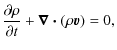
2.1 Equations
We solve the equations of magnetohydrodynamics (MHD) in the framework
of the shearing box model (Goldreich
& Lynden-Bell 1965) using two different codes: Athena
(Gardiner
& Stone 2005a,2008;
Stone
et al. 2008) and Ramses (Fromang
et al. 2006; Teyssier 2002).
Explicit microscopic
dissipation, namely viscosity ![]() and resistivity
and resistivity ![]() ,
are included in the simulations (note the microscopic
resistivity
,
are included in the simulations (note the microscopic
resistivity ![]() should not be confused with the turbulent resistivity
should not be confused with the turbulent resistivity
![]() that will be introduced below). It has been shown in the last few years
that both are
important in setting the saturated state of turbulence driven by the
MRI (Lesur
& Longaretti 2007; Fromang
et al. 2007). We use an isothermal equation of state
that will be introduced below). It has been shown in the last few years
that both are
important in setting the saturated state of turbulence driven by the
MRI (Lesur
& Longaretti 2007; Fromang
et al. 2007). We use an isothermal equation of state
![]() to relate
density
to relate
density ![]() and pressure P, where c0
is the sound speed. In a Cartesian coordinate system (x,y,z)
with unit vectors
and pressure P, where c0
is the sound speed. In a Cartesian coordinate system (x,y,z)
with unit vectors
![]() in the radial, azimuthal and vertical directions respectively, the
equations for mass and momentum conservation are:
in the radial, azimuthal and vertical directions respectively, the
equations for mass and momentum conservation are:
where
In order to study turbulent resistivity, we use a modified
form of the induction equation:
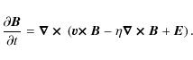
In this form we have introduced
|
(4) |
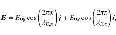
where
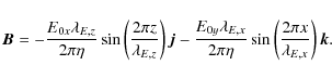
Equation (5) shows that the effect of the radial (x) component of the EMF is to create a vertically varying azimuthal magnetic field, while the effect of the azimuthal (y) component of the EMF is to create a radially varying vertical magnetic field. The amplitude of the field is determined by the amplitudes and wavelengths of the forcing and the resistivity. In a turbulent flow we expect the same balance will be achieved: turbulent velocity fluctuations will diffuse and reconnect the magnetic field that the driving EMF is trying to build. By analogy with Eq. (5), in a turbulent flow, we can define a turbulent resistivity

Similarly, the case E0x>0 and E0x=0 yields a purely azimuthal field varying with z and with an amplitude By0 that measures the turbulent resistivity

2.2 Numerical method
We solved Eqs. (1)-(3) using
Athena and Ramses in a box of size
(Lx,Ly,Lz)=(H,4H,H),
where ![]() defines
the vertical scale height (thickness) of the disk. We also used Athena
to compute a few runs with a larger extent in the radial direction:
(Lx,Ly,Lz)=(4H,4H,H).
It has been shown recently by Johnson
et al. (2008)
that truncation error in the shearing box can create numerical
artifacts, such as a density minima at the
center of the box (where the shear velocity with respect to the grid is
zero). We have implemented an orbital advection algorithm (Gammie 2001;
Johnson
& Gammie 2005; Johnson
et al. 2008; Masset
2000) in Athena
(Stone
& Gardiner 2009) to alleviate this problem, and at
the same time to allow for much larger timesteps in wide radial boxes.
defines
the vertical scale height (thickness) of the disk. We also used Athena
to compute a few runs with a larger extent in the radial direction:
(Lx,Ly,Lz)=(4H,4H,H).
It has been shown recently by Johnson
et al. (2008)
that truncation error in the shearing box can create numerical
artifacts, such as a density minima at the
center of the box (where the shear velocity with respect to the grid is
zero). We have implemented an orbital advection algorithm (Gammie 2001;
Johnson
& Gammie 2005; Johnson
et al. 2008; Masset
2000) in Athena
(Stone
& Gardiner 2009) to alleviate this problem, and at
the same time to allow for much larger timesteps in wide radial boxes.
All of our simulations are performed with no net magnetic flux in
either the vertical or azimuthal direction. At t=0,
we start with a purely vertical magnetic field varying sinusoidally
with x
so that the mean field vanishes. Random velocity perturbations of small
amplitude are applied to the background state, consisting of a uniform
density gas with a linear shear profile:
![]() .
We adopt
.
We adopt ![]() .
In the rest of this paper, we measure time in units of the orbital
period
.
In the rest of this paper, we measure time in units of the orbital
period ![]() .
In all of the simulations we present below, we set
.
In all of the simulations we present below, we set ![]() and
and ![]() such that the Reynolds number
such that the Reynolds number ![]() and the magnetic Prandtl number Pm=4. These
coefficients are identical to the run labeled 128Re3125Pm4
of Fromang
et al. (2007),
and are known to lead to sustained turbulence over large numbers of
orbital times. For explicit dissipation to dominate over numerical
dissipation, we used a resolution of 128 grid points
per H, or (Nx,Ny,Nz)=(128,512,128)
for calculations that span one scale height in the radial direction.
Such a resolution has been shown to give resolved solutions when using
2nd order Eulerian codes like ZEUS (Fromang
et al. 2007) for microscopic dissipation
coefficients
of the magnitude adopted here. Simon
et al. (2009)
have recently shown that the numerical dissipation in Athena, likely
comparable to Ramses, is similar in magnitude to that of ZEUS when
performing numerical simulations of MRI - induced
MHD turbulence in the shearing box. Thus, we expect the same
resolution needed with ZEUS is also appropriate for the runs presented
here that use
Athena or Ramses. In simulations with larger boxes, we scaled the
resolution accordingly,
(Nx,Ny,Nz)=(512,512,128),
so that the cell size remains the same.
and the magnetic Prandtl number Pm=4. These
coefficients are identical to the run labeled 128Re3125Pm4
of Fromang
et al. (2007),
and are known to lead to sustained turbulence over large numbers of
orbital times. For explicit dissipation to dominate over numerical
dissipation, we used a resolution of 128 grid points
per H, or (Nx,Ny,Nz)=(128,512,128)
for calculations that span one scale height in the radial direction.
Such a resolution has been shown to give resolved solutions when using
2nd order Eulerian codes like ZEUS (Fromang
et al. 2007) for microscopic dissipation
coefficients
of the magnitude adopted here. Simon
et al. (2009)
have recently shown that the numerical dissipation in Athena, likely
comparable to Ramses, is similar in magnitude to that of ZEUS when
performing numerical simulations of MRI - induced
MHD turbulence in the shearing box. Thus, we expect the same
resolution needed with ZEUS is also appropriate for the runs presented
here that use
Athena or Ramses. In simulations with larger boxes, we scaled the
resolution accordingly,
(Nx,Ny,Nz)=(512,512,128),
so that the cell size remains the same.
Regardless of the code we use or the size of the computational
domain, to study the turbulent resistivity induced by the MRI our
strategy is as follows: we first performed a run without forcing
(i.e.
![]() )
to let the MRI develop and for turbulence to reach a steady state.
Typically
these runs are evolved for 100 orbits. They also serve as a
useful
comparison between codes, and to compare small vs. large boxes.
At t=30,
we restarted the simulations with forcing of various amplitudes
imposed, as described above. With forcing, the flow evolves toward a
new quasi steady - state that we use to evaluate the turbulent
resistivity induced by the MRI. Before moving on to a description of
the results with forcing in Sect. 4, we
first describe the properties of MHD turbulence as obtained in
runs without forcing in the next section.
)
to let the MRI develop and for turbulence to reach a steady state.
Typically
these runs are evolved for 100 orbits. They also serve as a
useful
comparison between codes, and to compare small vs. large boxes.
At t=30,
we restarted the simulations with forcing of various amplitudes
imposed, as described above. With forcing, the flow evolves toward a
new quasi steady - state that we use to evaluate the turbulent
resistivity induced by the MRI. Before moving on to a description of
the results with forcing in Sect. 4, we
first describe the properties of MHD turbulence as obtained in
runs without forcing in the next section.
3 Runs without forcing
Table 1: Properties of MHD turbulence when forcing is turned off.
| Figure 1:
Time history of |
|
| Open with DEXTER | |
| Figure 2: Structure of the flow in the (x,z) plane obtained in model R-SB at t=70 orbits. The left, middle and right panels show the density, azimuthal component of the magnetic field, and vertical component of the velocity respectively. Similar results are obtained in model A-SB. |
|
| Open with DEXTER | |
![\begin{figure}
\par\includegraphics[width=14cm,clip]{12752f7.ps}\vspace*{0.15cm}...
...8.ps}\vspace*{0.15cm}
\includegraphics[width=14cm,clip]{12752f9.ps}
\end{figure}](/articles/aa/full_html/2009/43/aa12752-09/img44.png)
|
Figure 3: Same as Fig. 2 but for model A-LB: the upper, middle and lower panels show the density, azimuthal component of the magnetic field, and vertical component of the velocity respectively. |
| Open with DEXTER | |
| Figure 4: Space-time diagram showing the radial variation of the density, averaged along y and z, in model A-LB. It shows the appearance of long-lived density features. They are associated with large scale zonal flows as recently reported by Johansen et al. (2009). |
|
| Open with DEXTER | |
The parameters of the runs we present in this section, along
with
time averaged values from selected quantities measured from the runs,
are given in Table 1.
Each run is labeled according to the code used (``R'' for Ramses, or
``A'' for Athena) and the size of the box: ``SB'' for Small Box,
i.e. simulations performed with
( Lx,Ly,Lz)=(H,4H,H)
and ``LB'' for Large Box, i.e.
(Lx,Ly,Lz)=(4H,4H,H).
The resolution and duration of the runs are given in Cols. 3
and 4, respectively. In Col. 5, we report for each
model the
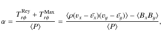
value of ![]() time averaged between t=50 and the end of the
simulation. As is usual, it is defined by the sum of the Reynolds and
Maxwell stress tensors,
time averaged between t=50 and the end of the
simulation. As is usual, it is defined by the sum of the Reynolds and
Maxwell stress tensors, ![]() and
and ![]() ,
normalized by the volume
averaged thermal pressure
,
normalized by the volume
averaged thermal pressure
![]() :
:
|
(8) |
where
We performed three runs. Two of them, R-SB and A-SB, share
identical
parameters but use different codes, Ramses and Athena respectively, in
order to compare the results from both codes. The third one, A-LB, was
performed with Athena in a larger domain. The last four columns of
Table 1
show that the saturated state of the turbulence is almost identical in
the three models. For example, ![]() ,
0.015 and 0.014 respectively in model R-SB,
A-SB and A-LB. This agreement is confirmed by the three panels of
Fig. 1
which correspond, from left to right, to R-SB, A-SB and A-LB. All show
the time history of
,
0.015 and 0.014 respectively in model R-SB,
A-SB and A-LB. This agreement is confirmed by the three panels of
Fig. 1
which correspond, from left to right, to R-SB, A-SB and A-LB. All show
the time history of ![]() (lower dashed line),
(lower dashed line), ![]() (upper dashed line) and
(upper dashed line) and ![]() (solid line). The curves obtained in the three
simulations are very similar and confirm the time averaged
(solid line). The curves obtained in the three
simulations are very similar and confirm the time averaged ![]() values
given in Table 1.
These results have two implications. First, the good agreement between
R-SB and A-SB gives confidence in both codes, as the two models have
identical parameters and differ only in the algorithms. Thus, it
validates both the implementation of the shearing box model in Ramses
and the implementation of orbital advection in Athena. Given the rms
fluctuations in
values
given in Table 1.
These results have two implications. First, the good agreement between
R-SB and A-SB gives confidence in both codes, as the two models have
identical parameters and differ only in the algorithms. Thus, it
validates both the implementation of the shearing box model in Ramses
and the implementation of orbital advection in Athena. Given the rms
fluctuations in ![]() reported in Table 1,
these results are also consistent with
the value of
reported in Table 1,
these results are also consistent with
the value of ![]() quoted by Fromang
et al. (2007) for their model 128Re3125Pm4.
We note, nonetheless, that the results obtained here with Athena and
Ramses appear to lead to slightly larger value of the angular momentum
transport. It is unclear (and beyond the scope of this paper) whether
this difference is significant. It may be partly due to our box size
being slightly larger in the azimuthal direction compared to that used
in Fromang
et al. (2007), or it
could
be due to small differences in the numerical dissipation between the
various codes. The second result that emerges from the models presented
in this section is the insensitivity of the turbulence properties to
the box size. The time averaged value of
quoted by Fromang
et al. (2007) for their model 128Re3125Pm4.
We note, nonetheless, that the results obtained here with Athena and
Ramses appear to lead to slightly larger value of the angular momentum
transport. It is unclear (and beyond the scope of this paper) whether
this difference is significant. It may be partly due to our box size
being slightly larger in the azimuthal direction compared to that used
in Fromang
et al. (2007), or it
could
be due to small differences in the numerical dissipation between the
various codes. The second result that emerges from the models presented
in this section is the insensitivity of the turbulence properties to
the box size. The time averaged value of ![]() in model A-LB is almost identical to the other two. The time
history presented on the right panel of Fig. 1
also shows good agreement with the other two panels. The only
difference is that the fluctuations around
the mean
in model A-LB is almost identical to the other two. The time
history presented on the right panel of Fig. 1
also shows good agreement with the other two panels. The only
difference is that the fluctuations around
the mean ![]() value
are smaller in the case of the big box. This translates into a standard
deviation which is about three times smaller in A-LB than in
the
other two models. Again, the reasons for this difference are unclear.
It may be due to better statistics in the large box (simply due to the
larger volume of the simulations) that average over extreme events.
Alternatively, it might be due to the larger number of parasitic modes
than can develop in larger boxes (Pessah
& Goodman 2009) or to a more efficient nonlinear
coupling between the more numerous turbulent modes present in a larger
box (Latter
et al. 2009).
Both effects would reduce the
lifetime (and therefore the influence) of channel modes. The similarity
between the small and large boxes model is further confirmed by
Figs. 2
and 3.
The
former shows snapshots of the density (left panel), By
(middle panel) and vz
(right panel) in the (x,z) plane
for model R-SB at t=70 (very similar
figures are obtained for model A-SB). The equivalent figures
for model A-LB at t=70 are shown in
Fig. 3.
The figure shows that the structure of the flow in the large box is
very similar to four patches of the small box model repeated next to
each other.
value
are smaller in the case of the big box. This translates into a standard
deviation which is about three times smaller in A-LB than in
the
other two models. Again, the reasons for this difference are unclear.
It may be due to better statistics in the large box (simply due to the
larger volume of the simulations) that average over extreme events.
Alternatively, it might be due to the larger number of parasitic modes
than can develop in larger boxes (Pessah
& Goodman 2009) or to a more efficient nonlinear
coupling between the more numerous turbulent modes present in a larger
box (Latter
et al. 2009).
Both effects would reduce the
lifetime (and therefore the influence) of channel modes. The similarity
between the small and large boxes model is further confirmed by
Figs. 2
and 3.
The
former shows snapshots of the density (left panel), By
(middle panel) and vz
(right panel) in the (x,z) plane
for model R-SB at t=70 (very similar
figures are obtained for model A-SB). The equivalent figures
for model A-LB at t=70 are shown in
Fig. 3.
The figure shows that the structure of the flow in the large box is
very similar to four patches of the small box model repeated next to
each other.
Other features typical of shearing box simulations of the MRI, like density wave propagating radially in the box (Heinemann & Papaloizou 2008a,b), are clearly seen in the density field regardless of the box size. Finally, as expected for a simulation having Pm>1, the smallest scale structure seen in the velocity field is generally larger than the smallest scale structure seen in the magnetic field. The latter shows elongated filaments reminiscent of high Pm small scale dynamo simulations (see for example Schekochihin et al. 2007).
Recently, Johansen
et al. (2009)
also reported numerical simulations of MHD turbulence in the
shearing box in large domains. They found an increase of ![]() when going from small (H) to
large (4H) boxes. Their result differs from
those reported here, where we find no sensitivity of
when going from small (H) to
large (4H) boxes. Their result differs from
those reported here, where we find no sensitivity of ![]() on box size. The reason probably lies in the fact that we always use
domains with an azimuthal extend of 4H,
even when the radial domain is small (i.e. when Lx
= H). On the
other hand, Johansen
et al. (2009) used square domains, with Lx
= Ly = H
in
their small box. It is well known that the azimuthal extent of
the
domain affects the saturated level of the turbulence (Hawley
et al. 1996,1995).
We conclude that, for fixed and large azimuthal extent of the domain,
the converged value of
on box size. The reason probably lies in the fact that we always use
domains with an azimuthal extend of 4H,
even when the radial domain is small (i.e. when Lx
= H). On the
other hand, Johansen
et al. (2009) used square domains, with Lx
= Ly = H
in
their small box. It is well known that the azimuthal extent of
the
domain affects the saturated level of the turbulence (Hawley
et al. 1996,1995).
We conclude that, for fixed and large azimuthal extent of the domain,
the converged value of ![]() is insensitive to the radial dimension of the box, at least for the
values of the Reynolds and Prandtl numbers studied here.
is insensitive to the radial dimension of the box, at least for the
values of the Reynolds and Prandtl numbers studied here.
Another property of the flow reported by Johansen et al. (2009) is the existence of large scale, long-lived zonal flows that generate axisymmetric density features in large boxes. We have looked for, and found, such features in our large box simulations as well. An example is shown in Fig. 4, a space-time diagram of the azimuthally and vertically averaged density in model A-LB. It is similar to Fig. 6 of Johansen et al. (2009) and shows a similar amplitude and lifetime for large scale density features, indicating that a zonal flows also develops in our simulations. As both results were obtained using completely different codes, our results confirm the conclusion drawn by Johansen et al. (2009): zonal flows appear to be a robust feature in MRI-driven turbulence in the shearing box.
This completes our description of the models computed in the
absence
of a forcing EMF. The flow in these models provides a starting point to
study turbulent resistivity induced by the MRI. Namely, at t=30,
we restarted the models using various amplitudes and directions for the
forcing EMF, ![]() .
The following section describe these results.
.
The following section describe these results.
4 Turbulent resistivity
Table 2: Properties of MHD turbulence when a forcing EMF is turned on.
The properties and results of the runs we performed are listed in
Table 2.
The first column gives a label for the name, coded according to the
following convention: ``direction-amplitude-code-parameters'' where
``direction'' can be either ``Ey'' or ``Ex'' and indicates the
direction of the forcing EMF (we considered only forcing aligned along
either the radial or the azimuthal direction, respectively creating
vertical or toroidal field), ``amplitude'' gives the amplitude of ![]() ,
``code'' reports the code we used for that model (``R'' for Ramses, and
``A'' for Athena), while ``parameters'', whenever present, gives
additional parameters that will be specified when needed in the text.
For example, model Ey-4E-10-R was performed with
Ramses using a forcing EMF in the azimuthal direction of amplitude
4
,
``code'' reports the code we used for that model (``R'' for Ramses, and
``A'' for Athena), while ``parameters'', whenever present, gives
additional parameters that will be specified when needed in the text.
For example, model Ey-4E-10-R was performed with
Ramses using a forcing EMF in the azimuthal direction of amplitude
4 ![]() 10-10. The other parameters reported in
Table 2
are the duration over which the data were
averaged (Col. 2), the amplitude of the forcing EMF
(Col. 3), the value of
10-10. The other parameters reported in
Table 2
are the duration over which the data were
averaged (Col. 2), the amplitude of the forcing EMF
(Col. 3), the value of ![]() (Col. 4) and the amplitude of the velocity fluctuations along
the three spatial coordinates (Cols. 5-7).
(Col. 4) and the amplitude of the velocity fluctuations along
the three spatial coordinates (Cols. 5-7).
The forcing EMF we imposed on the flow results in a
steady-state
magnetic field profile. We fitted the profile (averaged in time over
the duration of the run and in space over the two directions
perpendicular to the direction of variation) by a sinusoidal function.
The amplitude of the fit, ![]() ,
is expressed via the parameter
,
is expressed via the parameter

|
(9) |
and given in Col. 8 on Table 2. The turbulent resistivity
Finally, we follow Guan &
Gammie (2009) and associate a turbulent
``viscosity''
![]() with the flow, where
with the flow, where

|
(10) |
which we use to define a turbulent magnetic Prandtl number
4.1 Radial diffusion of a vertical magnetic field
4.1.1 E0y
= 4  10-10
10-10
![\begin{figure}
\par\includegraphics[width=7cm,clip]{12752f11.ps}\hspace*{3mm}
\i...
...13.ps}\hspace*{4mm}
\includegraphics[width=6.9cm,clip]{12752f14.ps}
\end{figure}](/articles/aa/full_html/2009/43/aa12752-09/img101.png)
|
Figure 5: Time averaged radial profile of the vertically and azimuthally averaged radial ( upper left panel), azimuthal ( upper right panel) and vertical ( lower left panel) magnetic field for model Ey-4E-10-R-LONG. On the third panel, the solid line shows the curve extracted from the numerical simulations while the dashed line is a least-squared fit to the data assuming a sinusoidal profile. The lower right panel shows the time variation of the standard deviation of the three magnetic field components, plotted using solid, dotted and dashed lines respectively. These plots illustrate that the forcing EMF creates, as expected, a radially varying vertical field with an amplitude larger than the fluctuations of the other magnetic field components. |
| Open with DEXTER | |
In this section, we describe in detail the results we obtained for
models Ey-4E-10-R, Ey-4E-10-R-LONG
and Ey-4E-10-A. All were obtained using a forcing
EMF directed along the
azimuthal direction, and varying only in the radial direction: E0x=0
and E0y=4 ![]() 10-10. We used
10-10. We used ![]() .
The first two were computed using Ramses and differ only in the
duration of the averaging procedure we applied. The third was computed
using Athena and serves both to validate our method and to quantify the
uncertainty in our estimate of the turbulent resistivity and magnetic
Prandtl number.
.
The first two were computed using Ramses and differ only in the
duration of the averaging procedure we applied. The third was computed
using Athena and serves both to validate our method and to quantify the
uncertainty in our estimate of the turbulent resistivity and magnetic
Prandtl number.
The results we obtained for this set of parameters are illustrated in
Fig. 5
for model Ey-4E-10-R-LONG.
There are four panels. The solid line in the first three (upper left,
upper right and lower left) plots the radial profile of Bx,
By and Bz
respectively,
averaged in time between t=30 and t=150
using 120 dumps, and averaged in space over y
and z.
All plots use the same vertical scale. It is apparent from the lower
left panel that the toroidal forcing EMF created a sinusoidally varying
vertical field, as expected from the discussion in Sect. 2. The dashed
line shows the sinusoidal curve obtained by a least square fit to the
data, and gives an amplitude ![]()
![]() 10-6 (this translates into a value
10-6 (this translates into a value ![]()
![]() 104 as shown in Table 2). It
is immediately obvious than this rather low value is mostly due to the
effect of turbulence. Indeed, using
Eq. (5),
the effect of the microscopic resistivity alone would give an amplitude
104 as shown in Table 2). It
is immediately obvious than this rather low value is mostly due to the
effect of turbulence. Indeed, using
Eq. (5),
the effect of the microscopic resistivity alone would give an amplitude
![]()
![]() 10-4, larger by about two orders of magnitude
than the measured value of the vertical field. Using Eq. (6), we
converted B0z
into a turbulent resistivity
10-4, larger by about two orders of magnitude
than the measured value of the vertical field. Using Eq. (6), we
converted B0z
into a turbulent resistivity ![]()
![]() 10-5. Combined with the time averaged value of
10-5. Combined with the time averaged value of ![]()
![]() 10-3, this gives a turbulent magnetic Prandtl
number of
10-3, this gives a turbulent magnetic Prandtl
number of
![]() .
.
Given the rather low value of the forcing EMF, it is
reasonable to
question the accuracy of these measurements. Indeed, the second and
third panels in Fig. 5
indicate that the
fluctuations in By
(upper right panel) are of comparable amplitude
to B0z![]() . The fourth (lower
right) panel, which shows the time history of the rms
fluctuations in the running time and spatial averages of Bz
(solid line) and By
(dashed line), indicates a similar trend: although
the rms fluctuations of Bz
become larger than those of By
after about 20 orbits (thus indicating than the standard
averaging
duration of 50 orbits we usually take in the following is
enough),
the ratio between the two is only a factor of about two after
120 orbits. In other words, the vertical field generated by
the
forcing EMF is not much larger than the turbulent fluctuations in the
field. As such, our measurements are susceptible to a rather
large
uncertainty
. The fourth (lower
right) panel, which shows the time history of the rms
fluctuations in the running time and spatial averages of Bz
(solid line) and By
(dashed line), indicates a similar trend: although
the rms fluctuations of Bz
become larger than those of By
after about 20 orbits (thus indicating than the standard
averaging
duration of 50 orbits we usually take in the following is
enough),
the ratio between the two is only a factor of about two after
120 orbits. In other words, the vertical field generated by
the
forcing EMF is not much larger than the turbulent fluctuations in the
field. As such, our measurements are susceptible to a rather
large
uncertainty![]() . In order to quantify this
uncertainty, we consider model Ey-4E-10-R,
which is the same as model Ey-4E-10-R-LONG
but averaged over only 50 orbits, and model Ey-4E-10-A,
identical to model Ey-4E-10-R but performed
using Athena. As shown on Table 2,
we found extremely close values for the turbulent resistivities for all
three models. The measured turbulent magnetic Prandtl number varies by
about
. In order to quantify this
uncertainty, we consider model Ey-4E-10-R,
which is the same as model Ey-4E-10-R-LONG
but averaged over only 50 orbits, and model Ey-4E-10-A,
identical to model Ey-4E-10-R but performed
using Athena. As shown on Table 2,
we found extremely close values for the turbulent resistivities for all
three models. The measured turbulent magnetic Prandtl number varies by
about ![]() ,
from
,
from ![]() to
to ![]() .
This difference can immediately be attributed to variations in the
measured
.
This difference can immediately be attributed to variations in the
measured ![]() ,
ranging from 1.7
,
ranging from 1.7 ![]() 10-3 to 2.3
10-3 to 2.3 ![]() 10-3. Such a variation is compatible with the
standard deviation of
10-3. Such a variation is compatible with the
standard deviation of ![]() reported in Table 1
and we conclude therefore that a safe estimate of the turbulent Prandtl
number in the radial direction in this case lies in the
range [1.,1.5].
reported in Table 1
and we conclude therefore that a safe estimate of the turbulent Prandtl
number in the radial direction in this case lies in the
range [1.,1.5].
This estimate is in rough agreement with the recent results reported by
Guan
& Gammie (2009) and Lesur
& Longaretti (2009)
in simulations performed in the presence of a net magnetic field in the
azimuthal or vertical direction. It is also reassuring that our
measured value for the turbulent resistivity is in rough agreement with
mean field theories like the Second-Order Correlation Approximation
(SOCA, Rädler
& Rheinhardt 2007) also known as the First Order
Smoothing Approximation (FOSA, Brandenburg
& Subramanian 2005). In this approach, the turbulent
resistivity is expected to take the form
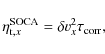
where
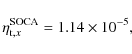
|
(12) |
a value that is, given the approximations involved in the SOCA, in very good agreement with the results reported in Table 2.
4.1.2 Varying the forcing EMFs
| Figure 6: Vertically, azimuthally and time averaged radial profile of the vertical magnetic field for models Ey-1E-9-R ( left panel), Ey-4E-9-R ( middle panel) and Ey-8E-9-R ( right panel). On each panel, the dashed line is a sinusoidal fit to the simulation data used to estimate the turbulent resistivities reported in Table 2. |
|
| Open with DEXTER | |
In the previous section, we considered a forcing whose
amplitude
only produces a very weak effect on the underlying turbulence. In this
section, we relax this hypothesis by considering larger forcing
EMFs. Such forcing may have an effect on the saturated properties of
the turbulence itself, which in turn may change the values of the
turbulent resistivity and
![]() .
.
In the run we performed, listed in Table 2, the
amplitude of the EMF was varied between ![]()
![]() 10-10 (described in the previous section) and
10-10 (described in the previous section) and ![]()
![]() 10-9, keeping
10-9, keeping ![]() in
all cases. We tried larger values as well
but found that, regardless of the code we used, the flow developed
regions of low density and large magnetic field. In these regions the
large Alfven speed resulted in an extremely small timestep, which
prevented the simulations from being continued.
in
all cases. We tried larger values as well
but found that, regardless of the code we used, the flow developed
regions of low density and large magnetic field. In these regions the
large Alfven speed resulted in an extremely small timestep, which
prevented the simulations from being continued.
Figure 6
shows the
radial profile (time averaged for 50 orbits and spatially
averaged
over the azimuthal and vertical directions) of the vertical magnetic
field we obtained in models Ey-1E-9-R (left
panel), Ey-4E-9-R (middle panel)
and Ey-8E-9-R (right panel). As
was the case for the lower left panel of Fig. 5, the
solid line plots the results of the simulation and the dashed line
shows the sinusoidal fit used to
derive the turbulent resistivity and magnetic Prandtl number. As
expected, Fig. 6
shows that the amplitude of the magnetic field increases with the
forcing amplitude. It also illustrates the quality of the sinusoidal
fit for these models. The turbulent resistivity and
magnetic Prandtl numbers we calculate using the amplitude of the
steady-state field are shown in Table 2. We
also report (Cols. 4 to 7) the time averaged ![]() values
and time averaged velocity fluctuations measured in these runs. As
forcing is increased, we find that
values
and time averaged velocity fluctuations measured in these runs. As
forcing is increased, we find that ![]() increases. Increasing the forcing by a a factor of 20
increases
increases. Increasing the forcing by a a factor of 20
increases ![]() by about 2.5. At the same time,
by about 2.5. At the same time, ![]() roughly triples.
This leads to a mild but systematic increase in
roughly triples.
This leads to a mild but systematic increase in ![]() with the amplitude of the forced vertical magnetic field.
To further test
our results, we also computed a model with
with the amplitude of the forced vertical magnetic field.
To further test
our results, we also computed a model with ![]()
![]() 10-9 with Athena (model Ey-4E-9-A
in Table 2).
The results are seen to be consistent with the results obtained with
Ramses.
10-9 with Athena (model Ey-4E-9-A
in Table 2).
The results are seen to be consistent with the results obtained with
Ramses.
![\begin{figure}
\par\includegraphics[width=8.5cm,clip]{12752f18.ps}
\end{figure}](/articles/aa/full_html/2009/43/aa12752-09/img121.png)
|
Figure 7: Turbulent resistivity in the radial direction as a function of the turbulent velocity fluctuations for various models computed using different amplitude of the forcing EMFs. Diamonds correspond to run performed using Ramses while stars use the results of models computed with Athena. The dotted line shows the prediction of SOCA assuming a constant correlation time, independent of the velocity fluctuations, while the dashed line shows the same prediction but computed assuming a correlation lengthscale for the magnetic field independent of the amplitude of the velocity fluctuations ( see text for details). The latter is seen to be in good agreement with the data. |
| Open with DEXTER | |
Since Eq. (11)
predicts the scaling of ![]() with the velocity fluctuations, in Fig. 7 we show
our results in the
with the velocity fluctuations, in Fig. 7 we show
our results in the ![]() plane.
The data obtained with Ramses are plotted using diamonds while the
points computed using Athena appear as a star symbol. The dotted line
is a naive estimate that uses the prediction of the SOCA given by
Eq. (11),
assuming that the correlation timescale is independent of the velocity
fluctuations:
plane.
The data obtained with Ramses are plotted using diamonds while the
points computed using Athena appear as a star symbol. The dotted line
is a naive estimate that uses the prediction of the SOCA given by
Eq. (11),
assuming that the correlation timescale is independent of the velocity
fluctuations: ![]() .
Clearly, the dotted line does not fit the
data. This is most likely because
.
Clearly, the dotted line does not fit the
data. This is most likely because ![]() varies as the strength of the turbulence changes. On dimensional
grounds, it can be estimated that
varies as the strength of the turbulence changes. On dimensional
grounds, it can be estimated that
where
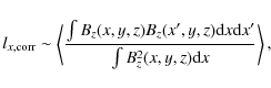
where angled brackets denote a spatial average over the y and z directions followed by a time average. Using Eq. (14), we found that

|
(15) |
where
|
(16) |
which we used to compute the dashed line shown in Fig. 7. The agreement with the data is much better and captures the scaling of the turbulent resistivity as the amplitude of the forcing EMFs is varied by more than one order of magnitude.
4.2 Radial diffusion of a vertical field in extended boxes
Next, we consider the turbulent resistivity in boxes extended
in the
radial direction. These models are based on the results of
model A-LB, which we restarted at time t=30
with forcing of
different amplitudes. We only consider forcing in the azimuthal
direction in this case. Again, we report the properties of the
turbulence and the values of
![]() and
and ![]() we obtained in Table 2.
we obtained in Table 2.
To check the results obtained in smaller boxes, we first consider
model Ey-4E-9-A-L4-lx1. In this case, we
used ![]() and E0y=4
and E0y=4 ![]() 10-10. Thus, it is the
big box equivalent of models Ey-4E-9-R and Ey-4E-9-A.
We therefore expect it to yield the same results. Table 2 shows
that this is indeed the case, with the values of
10-10. Thus, it is the
big box equivalent of models Ey-4E-9-R and Ey-4E-9-A.
We therefore expect it to yield the same results. Table 2 shows
that this is indeed the case, with the values of ![]() ,
,
![]() and
and ![]() being nearly the same in all three models.
being nearly the same in all three models.
Next, we turn to models Ey-4E-10-A-L4-lx4 and Ey-4E-9-A-L4-lx4
for which ![]() .
The first result to note is that the amplitude of the vertical field we
obtained is larger in these two cases than in the small box models with
equal forcing EMFs. This was somewhat expected. Since
.
The first result to note is that the amplitude of the vertical field we
obtained is larger in these two cases than in the small box models with
equal forcing EMFs. This was somewhat expected. Since
![]() is now larger, the local gradient of the vertical field are smaller in
the big boxes and the diffusion of magnetic field is less efficient.
Nevertheless, the measured turbulent resistivity are significantly
larger than their small boxes counterpart. At the same time, the
velocity fluctuations in the radial direction are comparable to the
small boxes models having the same forced vertical field amplitude. It
is likely that all other statistical properties of the
turbulence share the same insensitivity to box size, which means that a
straightforward application of the SOCA breaks down in this case. The
increased resistivity is therefore due to the increased
wavelength
is now larger, the local gradient of the vertical field are smaller in
the big boxes and the diffusion of magnetic field is less efficient.
Nevertheless, the measured turbulent resistivity are significantly
larger than their small boxes counterpart. At the same time, the
velocity fluctuations in the radial direction are comparable to the
small boxes models having the same forced vertical field amplitude. It
is likely that all other statistical properties of the
turbulence share the same insensitivity to box size, which means that a
straightforward application of the SOCA breaks down in this case. The
increased resistivity is therefore due to the increased
wavelength
![]() of the forcing EMF used in that case. One possible explanation, to be
taken with care, for such large
of the forcing EMF used in that case. One possible explanation, to be
taken with care, for such large
![]() can
then be described as follows: the resulting forced magnetic field,
having a larger scale, will most likely be diffused by larger eddies.
Because the kinetic energy power spectrum is decreasing with
wavenumber, such eddies have a larger
kinetic energy that makes them more efficient at diffusing the magnetic
field.
can
then be described as follows: the resulting forced magnetic field,
having a larger scale, will most likely be diffused by larger eddies.
Because the kinetic energy power spectrum is decreasing with
wavenumber, such eddies have a larger
kinetic energy that makes them more efficient at diffusing the magnetic
field.
The consequence of the larger turbulent resistivities obtained in our
large box simulations is lower values of ![]() .
In the case of model Ey-4E-10-A-L4-lx4,
.
In the case of model Ey-4E-10-A-L4-lx4, ![]() ,
i.e. a factor of about three times smaller compared to the
small boxes. We recover
,
i.e. a factor of about three times smaller compared to the
small boxes. We recover ![]() of order unity for model Ey-4E-9-A-L4-lx4 owing to
a larger value of
of order unity for model Ey-4E-9-A-L4-lx4 owing to
a larger value of ![]() .
This is presumably due to the fact that the flow starts to behave as if
threaded by a net vertical flux for this long wavelength, large
amplitude forcing.
.
This is presumably due to the fact that the flow starts to behave as if
threaded by a net vertical flux for this long wavelength, large
amplitude forcing.
4.3 Vertical diffusion of an azimuthal magnetic field
In addition to studying radial diffusion of vertical magnetic
fields
as described in the previous section, we also performed simulations in
which we study the vertical diffusion of an azimuthal magnetic field.
In this case, we restricted our analysis to small boxes, and we chose
E0y=0 and
therefore considered forcing EMFs
purely in the radial direction. We allowed for variations of the
amplitude of the forcing in the range 4 ![]() 10-9<E0x<
8
10-9<E0x<
8 ![]() 10-9. We also tried E0x=4
10-9. We also tried E0x=4 ![]() 10-10
as in the case of radial diffusion. However, because the azimuthal
magnetic field fluctuations are of larger amplitudes than the vertical
field fluctuations, it has proven difficult to extract a meaningful
mean field from that model. We therefore decided to consider only large
amplitudes for the forcing EMFs.
10-10
as in the case of radial diffusion. However, because the azimuthal
magnetic field fluctuations are of larger amplitudes than the vertical
field fluctuations, it has proven difficult to extract a meaningful
mean field from that model. We therefore decided to consider only large
amplitudes for the forcing EMFs.
The results we obtained are summarized once more in Table 2.
We obtain turbulent resisitivities that are generally lower than for
the case of radial field diffusion. This is
not inconsistent with the prediction of SOCA, as the velocity
fluctuations in the vertical direction are of lower amplitudes than the
velocity fluctuations in the radial direction. Using
we obtained
Finally, because of the lower values of the turbulent
resistivity, the final column of Table 2
reports systematically larger values of the turbulent magnetic Prandtl
number, ranging from 1.57 for model Ex-4E-9-R
to 3.00 for model Ex-4E-9-R. As in
the case of a vertical field diffusing radially, ![]() is
a slowly increasing function of the strength of the turbulence.
is
a slowly increasing function of the strength of the turbulence.
5 Discussion and conclusion
In this paper, we have presented a set of local numerical
simulations aimed at measuring the properties of turbulent diffusion of
magnetic field, quantified using an anomalous turbulent
resistivity
![]() ,
resulting from MHD turbulence induced by the MRI. We
considered
only
the case in which turbulence develops in the absence of a mean magnetic
field. We used two different codes, Athena and Ramses, and vary both
the box size and the magnetic field geometry. The main result that
emerges from our simulations is that
,
resulting from MHD turbulence induced by the MRI. We
considered
only
the case in which turbulence develops in the absence of a mean magnetic
field. We used two different codes, Athena and Ramses, and vary both
the box size and the magnetic field geometry. The main result that
emerges from our simulations is that
![]() tends to be slightly smaller,
but similar in magnitude, to the anomalous viscosity
tends to be slightly smaller,
but similar in magnitude, to the anomalous viscosity
![]() that can be associated with the outward transport of angular momentum
due to the turbulence. In other words, their ratio, the turbulent
magnetic number
that can be associated with the outward transport of angular momentum
due to the turbulence. In other words, their ratio, the turbulent
magnetic number
![]() ,
is of order unity (actually in most of our runs it was slightly larger
than one). We also found that our results are roughly consistent with
the predictions of the mean field theory SOCA. Perhaps more relevant is
the fact that our results are consistent with those recently published
by Guan
& Gammie (2009) and Lesur
& Longaretti (2009),
who used different field topologies (toroidal and vertical mean field),
different numerical methods (similar to those in the ZEUS code, and an
incompressible pseudo-spectral code respectively) and, as described in
the introduction, different approaches to measure the turbulent
resistivity. This broad agreement demonstrates that all these results,
obtained and published independently, are largely insensitive to the
numerical method and the topogoly of the magnetic field.
As suggested already in the literature (Parker 1971),
a safe first order guess of the magnitude of the turbulent resistivity
is therefore
,
is of order unity (actually in most of our runs it was slightly larger
than one). We also found that our results are roughly consistent with
the predictions of the mean field theory SOCA. Perhaps more relevant is
the fact that our results are consistent with those recently published
by Guan
& Gammie (2009) and Lesur
& Longaretti (2009),
who used different field topologies (toroidal and vertical mean field),
different numerical methods (similar to those in the ZEUS code, and an
incompressible pseudo-spectral code respectively) and, as described in
the introduction, different approaches to measure the turbulent
resistivity. This broad agreement demonstrates that all these results,
obtained and published independently, are largely insensitive to the
numerical method and the topogoly of the magnetic field.
As suggested already in the literature (Parker 1971),
a safe first order guess of the magnitude of the turbulent resistivity
is therefore ![]() .
.
A number of other results emerge from the comparison of the suite of
simulations we present here with the work of Guan &
Gammie (2009) and Lesur
& Longaretti (2009). First, it is worth noting that
our results and those of Lesur
& Longaretti (2009) were obtained including explicit
dissipation, while those of Guan &
Gammie (2009)
relied only on numerical dissipation. Since all the results are roughly
consistent with one another, this is apparently not an issue as far as
determining ![]() is concerned. Moreover, Lesur
& Longaretti (2009) consider the case Pm=1
while we have used Pm=4. The broad agreement
between both studies therefore suggest that
is concerned. Moreover, Lesur
& Longaretti (2009) consider the case Pm=1
while we have used Pm=4. The broad agreement
between both studies therefore suggest that
![]() does not strongly depend on microscopic dissipation coefficients.
However, it would be premature to draw definite statements here since
other differences between both works might mask a possible Pm dependence
in the results. Although very computationally expensive, a systematic
study of the
sensitivity of our results to the value of Pm is
needed in the future. Second,
does not strongly depend on microscopic dissipation coefficients.
However, it would be premature to draw definite statements here since
other differences between both works might mask a possible Pm dependence
in the results. Although very computationally expensive, a systematic
study of the
sensitivity of our results to the value of Pm is
needed in the future. Second, ![]() appears to be smaller in large boxes. Indeed, we found
appears to be smaller in large boxes. Indeed, we found ![]() for model Ey-4E-10-A-L4-lx4, while
for model Ey-4E-10-A-L4-lx4, while ![]() is found to be larger than one in small boxes having identical
parameters. This rather low value, obtained in a large box and for a
small forcing EMF, is very close to the values quoted by Guan &
Gammie (2009) for models having the same radial box size and
a weak imposed field. In addition, Guan &
Gammie (2009) considered boxes larger than 4H
in the radial direction and found this value of
is found to be larger than one in small boxes having identical
parameters. This rather low value, obtained in a large box and for a
small forcing EMF, is very close to the values quoted by Guan &
Gammie (2009) for models having the same radial box size and
a weak imposed field. In addition, Guan &
Gammie (2009) considered boxes larger than 4H
in the radial direction and found this value of ![]() to be independent of box size. By contrast, both our results and those
of Lesur
& Longaretti (2009) suggest a value larger than one
(or equivalently fairly low values for the turbulent resisitivity) in
small boxes, a regime Guan
& Gammie (2009) did not investigate. Taken together,
all these results point toward a decrease of
to be independent of box size. By contrast, both our results and those
of Lesur
& Longaretti (2009) suggest a value larger than one
(or equivalently fairly low values for the turbulent resisitivity) in
small boxes, a regime Guan
& Gammie (2009) did not investigate. Taken together,
all these results point toward a decrease of ![]() when box size is increased from values of a few to values of roughly
one half, with a plateau obtained for boxes larger than 4H.
when box size is increased from values of a few to values of roughly
one half, with a plateau obtained for boxes larger than 4H.
Despite their broad agreement, it is instructive to consider the
differences between our results and the aformentionned papers (Lesur
& Longaretti 2009; Guan &
Gammie 2009). One such difference is that,
regardless of the model or the box size, we always find that ![]() increases with the amplitude of the forcing EMF. Lesur
& Longaretti (2009) also report such a trend for the
models they label XXZn, in which they consider the vertical diffusion
of a toroidal field, as we do in Sect. 4.3.
These trend is not so clear for their other cases. However, most of
their runs were obtained in the presence of a net vertical flux. The
nature of the turbulence is strongly modified in that case and this is
probably not appropriate to draw the comparison with those models any
further. By contrast, Guan
& Gammie (2009) report no dependence of
increases with the amplitude of the forcing EMF. Lesur
& Longaretti (2009) also report such a trend for the
models they label XXZn, in which they consider the vertical diffusion
of a toroidal field, as we do in Sect. 4.3.
These trend is not so clear for their other cases. However, most of
their runs were obtained in the presence of a net vertical flux. The
nature of the turbulence is strongly modified in that case and this is
probably not appropriate to draw the comparison with those models any
further. By contrast, Guan
& Gammie (2009) report no dependence of
![]() on the amplitude of the magnetic field they impose for models that are
similar to ours (i.e. the diffusion of a radially varying
vertical
field). Even if the different field topology they consider (namely a
net toroidal flux) plays a role, the difference with our results can
most likely be attributed to the different methods that are being used.
While the present paper aims to measure a steady state response of the
flow to a perturbation that is imposed at all times, Guan &
Gammie (2009) superpose an additional field to an already
turbulent flow at t=0
and let it decay. Thus it is possible that transients associated with
this additional field may complicate the estimate of time averaged
values for the transport coefficients
on the amplitude of the magnetic field they impose for models that are
similar to ours (i.e. the diffusion of a radially varying
vertical
field). Even if the different field topology they consider (namely a
net toroidal flux) plays a role, the difference with our results can
most likely be attributed to the different methods that are being used.
While the present paper aims to measure a steady state response of the
flow to a perturbation that is imposed at all times, Guan &
Gammie (2009) superpose an additional field to an already
turbulent flow at t=0
and let it decay. Thus it is possible that transients associated with
this additional field may complicate the estimate of time averaged
values for the transport coefficients![]() .
In particular, for large strength of the additional field, the flow may
not have enough time to reach fully saturated values of the turbulence
before the strength of the imposed field decays significantly. This
might lead to an underestimate of the value of
.
In particular, for large strength of the additional field, the flow may
not have enough time to reach fully saturated values of the turbulence
before the strength of the imposed field decays significantly. This
might lead to an underestimate of the value of ![]() and consequently of the value of
and consequently of the value of ![]() ,
masking the increase of
,
masking the increase of ![]() with forcing that we found.
with forcing that we found.
It is also important to stress that all three approaches share common limitations to their analyses. First and foremost, the analysis is by definition local, whereas the diffusion of magnetic field accross the disk is an intrisically global problem that depends on the large scale properties of the disk such as the radial profiles of the surface density and magnetic flux (Spruit & Uzdensky 2005). Another related limitation is the neglect of vertical density stratification in the disk. Indeed, all three studies presents numerical simulations performed in ``unstratified'' shearing boxes, neglecting the vertical component of gravity. In simulations including gas density stratification, it was found that MHD turbulence is suppressed in the low density corona above and below the disk midplane (Stone et al. 1996). It is likely that turbulent diffusion will be greatly reduced at those locations, possibly causing the magnetic flux to remain anchored to the disk corona. This could prevent diffusion that otherwise would have been driven by turbulence in the midplane, or by channel modes that couple the upper layers of the disk with the midplane (Lovelace et al. 2009; Rothstein & Lovelace 2008; Bisnovatyi-Kogan & Lovelace 2007). A numerical test of this scenario is beyong the scope of the present paper but should be considered in the future. Finally, let us mention the very recent work of Beckwith et al. (2009). Using global simulations that combine the large scale nature of magnetic field diffusion and the vertical density stratication (but, of course, with a dramatic reduction in the spatial resolution), these authors challenge the concept of turbulent resistivity itself and advocate a completely different scenario to describe magnetic flux evolution in accretion disks. Clearly, despite the agreement with already published calculations, the results presented here should be taken with care when used in the context of astrophysical applications, such as jet launching or magnetic flux distribution in accretion disks.
AcknowledgementsWe thank J. Goodman for suggesting the method used in this paper to measure the turbulent resistivity, and G. Lesur and P.-Y. Longaretti for stimulating discussions. S.F. acknowledges the Astronomy Department of Princeton University and the Institute of Advanced Studies for their hospitality during visits that enabled this work to be initiated. This work used the computational facilities supported by the Princeton Institute for Computational Science and Engineering.
References
- Balbus, S., & Hawley, J. 1991, ApJ, 376, 214 [CrossRef] [NASA ADS]
- Balbus, S., & Hawley, J. 1998, Rev. Mod. Phys., 70, 1 [CrossRef] [NASA ADS]
- Beckwith, K., Hawley, J. F., & Krolik, J. H. 2009, arXiv e-prints
- Bisnovatyi-Kogan, G. S., & Lovelace, R. V. E. 2007, ApJ, 667, L167 [CrossRef] [NASA ADS]
- Blandford, R. D., & Payne, D. G. 1982, MNRAS, 199, 883 [NASA ADS]
- Brandenburg, A., & Subramanian, K. 2005, Phys. Rep., 417, 1 [CrossRef] [NASA ADS]
- Casse, F., & Ferreira, J. 2000, A&A, 353, 1115 [NASA ADS]
- Fromang, S., & Nelson, R. P. 2009, A&A, 496, 597 [EDP Sciences] [CrossRef] [NASA ADS]
- Fromang, S., & Papaloizou, J. 2006, A&A, 452, 751 [EDP Sciences] [CrossRef] [NASA ADS]
- Fromang, S., Hennebelle, P., & Teyssier, R. 2006, A&A, 457, 371 [EDP Sciences] [CrossRef] [NASA ADS]
- Fromang, S., Papaloizou, J., Lesur, G., & Heinemann, T. 2007, A&A, 476, 1123 [EDP Sciences] [CrossRef] [NASA ADS]
- Gammie, C. F. 2001, ApJ, 553, 174 [CrossRef] [NASA ADS]
- Gardiner, T. A., & Stone, J. M. 2005a, J. Comput. Phys., 205, 509 [CrossRef] [NASA ADS]
- Gardiner, T. A., & Stone, J. M. 2005b, in Magnetic Fields in the Universe: From Laboratory and Stars to Primordial Structures., ed. E. M. de Gouveia dal Pino, G. Lugones, & A. Lazarian, AIP Conf. Proc., 784, 475
- Gardiner, T. A., & Stone, J. M. 2008, J. Comput. Phys., 227, 4123 [CrossRef] [NASA ADS]
- Goldreich, P., & Lynden-Bell, D. 1965, MNRAS, 130, 125 [NASA ADS]
- Guan, X., & Gammie, C. F. 2009, ApJ, 697, 1901 [CrossRef] [NASA ADS]
- Guan, X., Gammie, C. F., Simon, J. B., & Johnson, B. M. 2009, ApJ, 694, 1010 [CrossRef] [NASA ADS]
- Hawley, J., & Stone, J. 1995, Comput. Phys. Commun., 89, 127 [CrossRef] [NASA ADS]
- Hawley, J. F., Gammie, C. F., & Balbus, S. A. 1995, ApJ, 440, 742 [CrossRef] [NASA ADS]
- Hawley, J. F., Gammie, C. F., & Balbus, S. A. 1996, ApJ, 464, 690 [CrossRef] [NASA ADS]
- Heinemann, T., & Papaloizou, J. C. B. 2008a, MNRAS, 397, 52 [CrossRef] [NASA ADS]
- Heinemann, T., & Papaloizou, J. C. B. 2008b, MNRAS, 397, 64 [CrossRef] [NASA ADS]
- Johansen, A., Youdin, A., & Klahr, H. 2009, ApJ, 697, 1269 [CrossRef] [NASA ADS]
- Johnson, B. M., & Gammie, C. F. 2005, ApJ, 635, 149 [CrossRef] [NASA ADS]
- Johnson, B. M., Guan, X., & Gammie, C. F. 2008, ApJS, 177, 373 [CrossRef] [NASA ADS]
- Landau, L. D., & Lifshitz, E. M. 1959, Fluid mechanics, Course of theoretical physics (Oxford: Pergamon Press)
- Latter, H. N., Lesaffre, P., & Balbus, S. A. 2009, MNRAS, 394, 715 [CrossRef] [NASA ADS]
- Lesur, G., & Longaretti, P.-Y. 2007, MNRAS, 378, 1471 [CrossRef] [NASA ADS]
- Lesur, G., & Longaretti, P.-Y. 2009, A&A, 504, 309 [EDP Sciences] [CrossRef]
- Lovelace, R. V. E., Bisnovatyi-Kogan, G. S., & Rothstein, D. M. 2009, Nonlinear Processes in Geophys., 16, 77 [NASA ADS]
- Lubow, S. H., Papaloizou, J. C. B., & Pringle, J. E. 1994, MNRAS, 267, 235 [NASA ADS]
- Masset, F. 2000, A&AS, 141, 165 [EDP Sciences] [CrossRef] [NASA ADS]
- Parker, E. N. 1971, ApJ, 163, 279 [CrossRef] [NASA ADS]
- Pessah, M. E., & Goodman, J. 2009, ApJ, 698, 72 [CrossRef] [NASA ADS]
- Pudritz, R. E., Ouyed, R., Fendt, C., & Brandenburg, A. 2007, in Protostars and Planets V, ed. B. Reipurth, D. Jewitt, & K. Keil, 277
- Rädler, K.-H., & Rheinhardt, M. 2007, Geophys. Astrophys. Fluid Dyn., 101, 117 [CrossRef] [NASA ADS]
- Rothstein, D. M., & Lovelace, R. V. E. 2008, ApJ, 677, 1221 [CrossRef] [NASA ADS]
- Schekochihin, A. A., Iskakov, A. B., Cowley, S. C., et al. 2007, New J. Phys., 9, 300 [CrossRef]
- Shakura, N. I., & Sunyaev, R. A. 1973, A&A, 24, 337 [NASA ADS]
- Simon, J. B., Hawley, J. F., & Beckwith, K. 2009, ApJ, 690, 974 [CrossRef] [NASA ADS]
- Spruit, H. C., & Uzdensky, D. A. 2005, ApJ, 629, 960 [CrossRef] [NASA ADS]
- Stone, J. M., & Norman, M. L. 1992, ApJS, 80, 791 [CrossRef] [NASA ADS]
- Stone, J. M., & Gardiner, T. A. 2009, ApJ, in preparation
- Stone, J. M., Hawley, J. F., Gammie, C. F., & Balbus, S. A. 1996, ApJ, 463, 656 [CrossRef] [NASA ADS]
- Stone, J. M., Gardiner, T. A., Teuben, P., Hawley, J. F., & Simon, J. B. 2008, ApJS, 178, 137 [CrossRef] [NASA ADS]
- Teyssier, R. 2002, A&A, 385, 337 [EDP Sciences] [CrossRef] [NASA ADS]
- van Ballegooijen, A. A. 1989, in Accretion Disks and Magnetic Fields in Astrophysics, ed. G. Belvedere, Astrophys. Space Sci. Library, 156, 99
Footnotes
- ...B
![[*]](/icons/foot_motif.png)
- The absence of fluctuations in the y and z averaged radial profile of Bx comes from the solenoidal nature of the magnetic field.
- ... uncertainty
- The reason to study such small fields is so that they do
not significantly affect the property of the turbulence itself
(the wavelength of the most unstable wavelength of the MRI associated
with the field generated by the forcing EMF is largely underesolved in
our simulations). Thus, they merely act as a passive probe of the
turbulence, which is not the case for the larger amplitude of
 we consider
in Sect. 4.1.2.
we consider
in Sect. 4.1.2.
- ... coefficients
- Of course, such transients are most likely of physical
origin, in the sense that the decay timescale measured by Guan &
Gammie (2009)
is related to the relaxation timescale of the turbulence. Nevertheless,
their presence complicate the estimate of

All Tables
Table 1: Properties of MHD turbulence when forcing is turned off.
Table 2: Properties of MHD turbulence when a forcing EMF is turned on.
Current usage metrics show cumulative count of Article Views (full-text article views including HTML views, PDF and ePub downloads, according to the available data) and Abstracts Views on Vision4Press platform.
Data correspond to usage on the plateform after 2015. The current usage metrics is available 48-96 hours after online publication and is updated daily on week days.
Initial download of the metrics may take a while.