| Issue |
A&A
Volume 509, January 2010
|
|
|---|---|---|
| Article Number | A43 | |
| Number of page(s) | 11 | |
| Section | Stellar atmospheres | |
| DOI | https://doi.org/10.1051/0004-6361/200912239 | |
| Published online | 15 January 2010 | |
Surface structure of the CoRoT CP2 target star HD 50773![[*]](/icons/foot_motif.png)
T. Lüftinger1 - H.-E. Fröhlich2 - W. W. Weiss1 - P. Petit3 - M. Aurière3 - N. Nesvacil1 - M. Gruberbauer1 - D. Shulyak1 - E. Alecian4 - A. Baglin4 - F. Baudin7 - C. Catala4 - J.-F. Donati3 - O. Kochukhov5 - E. Michel4,6 - N. Piskunov5 - T. Roudier3 - R. Samadi4,6
1 - Institut für Astronomie, Universität Wien, Türkenschanzstrasse 17, 1180 Wien, Austria
2 - Astrophysikalisches Institut Potsdam, An der Sternwarte 16, 14482 Potsdam, Germany
3 - Laboratoire d'Astrophysique de Toulouse-Tarbes, Université de Toulouse, CNRS, France
4 - Observatoire de Paris, LESIA, 5 place Jules Janssen, 92195 Meudon Cedex, France
5 - Department of Physics and Astronomy, Uppsala University, 75120 Uppsala, Sweden
6 - Université Pierre et Marie Curie, Université Denis Diderot, Pl. J. Janssen, 92195 Meudon, France
7 - Institut d'Astrophysique Spatiale, UMR8617, Université Paris X, Bât. 121, 91405 Orsay, France
Received 31 March 2009 / Accepted 27 October 2009
Abstract
Aims. We compare surface maps of the chemically peculiar
star HD 50773 produced with a Bayesian technique and based on high
quality CoRoT photometry with those derived from rotation phase
resolved spectropolarimetry. The goal is to investigate the correlation
of surface brightness with surface chemical abundance distribution and
the stellar magnetic surface field.
Methods. The rotational period of the star was determined from a
nearly 60 days long continuous light curve obtained during the
initial run of CoRoT. Using a Bayesian approach to star-spot modelling,
which in this work is applied for the first time for the photometric
mapping of a CP star, we derived longitudes, latitudes and
radii of four different spot areas. Additional parameters like stellar
inclination and the spot's intensities were also determined. The CoRoT
observations triggered an extensive ground-based spectroscopic and
spectropolarimetric observing campaign and enabled us to obtain
19 different high resolution spectra in Stokes parameters I and V
with NARVAL, ESPaDOnS, and SemelPol spectropolarimeters. Doppler and
Magnetic Doppler imaging techniques allowed us to derive the
magnetic field geometry of the star and the surface abundance
distributions of Mg, Si, Ca, Ti, Cr, Fe, Ni, Y, and Cu.
Results. We find a dominant dipolar structure of the surface
magnetic field. The CoRoT light curve variations and abundances of most
elements mapped are correlated with the aforementioned
geometry: Cr, Fe, and Si are enhanced around the magnetic
poles and coincide with the bright regions on the surface
of HD 50773 as predicted by our light curve synthesis and
confirmed by photometric imaging.
Key words: stars: atmospheres - stars: chemically peculiar - stars: individual: HD 50773 - stars: magnetic field - stars: imaging
1 Introduction
CoRoT (Convection, Rotation and planetary Transits) is a space mission with the participation of ESA's Science Program and Research and Scientific Support Department (RSSD), Austria, Belgium, Brazil, Germany, and Spain. It focuses on high precision photometry from space, also taking advantage of observing given targets continuously during nearly half a year, which is impossible from the ground. A technical overview is presented in Boisnard & Auvergne (2006), and the asteroseismology related mission aspects are discussed in Baglin et al. (2006) and references therein.
HD 50773 (BD -00 1488, TYC 4801-2-1, mag(B) = 9.50) was observed during the initial run of CoRoT only little more than a month after the launch on December 27, 2006, on board of a Soyuz Fregat II-1b. The star was chosen in the seismology field as one of ten possible targets because of its location in the classical instability strip and of its suspected chemical peculiarity. The reduction of the CoRoT photometry to the N2 data format is described in Appourchaux et al. (2008), and our additional reduction steps are given in Sect. 2 of this paper.
Not much has been published about this star, which is classified in SIMBAD as an A2 star and as an A4-A9 suspected chemically peculiar star in Renson et al. (1991) with so far no measured magnetic field nor rotation period.
Magnetic Ap stars, to which HD 50773 belongs, represent about 1% to 5% of the upper main sequence stars and exhibit highly ordered, very stable and often very strong magnetic fields. They frequently show both brightness- and spectral line profile variations synchronised to stellar rotation. These variations are hitherto most successfully explained by the oblique rotator model (introduced by Stibbs 1950) and are attributed to oblique magnetic and rotation axes and to the presence of a non-uniform distribution of chemical elements on their surface.
The abundance inhomogeneities in turn are said to arise from the selective diffusion of ions under the competitive action of radiative acceleration and gravitational settling (Michaud 1970) under the influence of the (oblique) magnetic field, possibly in combination with a weak stellar wind (see, e.g., Babel 1992).
The light curve of HD 50773 obtained by CoRoT has a double wave
form with two clear maxima of slightly different amplitudes at phases
of ![]()
![]() 0.05 and 0.52 (see Fig. 1).
This photometric variability is, as mentioned, likely to be connected
with the inhomogeneous surface element distribution as shown in e.g.,
Krticka et al. (2007) and references therein. As the star seems to be of the Cr CP2-type, we expect
brighter spots rather than dark ones (see e.g. Mikulásek et al. 2007, 2008a,b).
Bright photometric spots seem to be closely connected with
overabundance regions
of Si or Fe, and the mechanism of the origin of their
contrast in the optical spectrum region is well described in Krticka
et al. (2009).
0.05 and 0.52 (see Fig. 1).
This photometric variability is, as mentioned, likely to be connected
with the inhomogeneous surface element distribution as shown in e.g.,
Krticka et al. (2007) and references therein. As the star seems to be of the Cr CP2-type, we expect
brighter spots rather than dark ones (see e.g. Mikulásek et al. 2007, 2008a,b).
Bright photometric spots seem to be closely connected with
overabundance regions
of Si or Fe, and the mechanism of the origin of their
contrast in the optical spectrum region is well described in Krticka
et al. (2009).
![\begin{figure}
\par\includegraphics[width=8.8cm,clip]{12239fg1.ps}
\vspace*{5mm}
\end{figure}](/articles/aa/full_html/2010/01/aa12239-09/img8.png)
|
Figure 1: Phase plot of HD 50773 using a binned light curve after the subtraction of effects due to the CoRoT orbit and the stellar signal not attributed to rotation. Overplotted (white line) is the four-spot model fit described in Sect. 4 of this paper. |
| Open with DEXTER | |
It is still not understood why some of the upper main sequence stars are magnetic and chemically peculiar and others are not, where the magnetic fields of CP2 stars originate from, and how these fields exactly interplay and correlate with the inhomogeneous surface distribution of chemical elements. Deriving in detail the surface structure of HD 50773 in the way presented in this paper will contribute to solving this puzzle.
Our paper is organised in Sect. 2, where we present our CoRoT space photometry, spectropolarimetric observations, and the data reduction, while the physical parameters of the target star HD 50773 and a detailed abundance analysis are presented in Sect. 3. In Sect. 4 we discuss our analysis of the surface structure of HD 50773 by applying Bayesian methods to the CoRoT light curve. Details about the magnetic field geometry and the surface abundance structures of individual elements are presented in Sects. 5 and 6. In Sect. 7 we discuss the theoretical predictions of light variability, taking into account the surface abundance inhomogeneities, and Sect. 8 is devoted to the comparison of our different approaches and the discussion of results.
2 Observations and data reduction
2.1 CoRoT data
HD 50773 was observed by CoRoT from February 3 to April 2, 2007. The reduction of the CoRoT photometry to the N2 level was performed as described in Appourchaux et al. (2008). The time span of 57.7 days covers 27.6 stellar rotational cycles, and the overall variation in brightness amounts to 0.017 mag. The wavelength range (in the CoRoT seismology field) defined by the CoRoT photometric CCD covers 2500 Å to 11 000 Å. For additonal instrumental details, we kindly refer the reader to Fridlund et al. (2006).
Any instrumental signal or stellar variation not associated with
rotation and not consistent with Gaussian noise or a linear trend would
affect the determination of the various parameters in our spot model.
Therefore, we tested the light curve for any jumps in flux,
which could either be caused by the star itself or the instrument. We
first subtracted
a linear trend from the time series attributed to aging effects in the
detector and electronics chain (Auvergne et al. 2009) and
subsequently removed the apparent stellar rotational variability from
the data. Low-order polynomials were fitted to short subsets
![]() of the residual data in order to eliminate the signal changes due to
rotation, which resulted in a residual time series shown in the upper
panel of Fig. 2.
In a next step we calculated a running average of this residual
time series using a box width of 370 data points and subtracted
the running average - resampled to the original time tags -
from the original light curve.
The result is shown in the lower panel of Fig. 2.
of the residual data in order to eliminate the signal changes due to
rotation, which resulted in a residual time series shown in the upper
panel of Fig. 2.
In a next step we calculated a running average of this residual
time series using a box width of 370 data points and subtracted
the running average - resampled to the original time tags -
from the original light curve.
The result is shown in the lower panel of Fig. 2.
The upper panel of Fig. 3
shows the original CoRoT light curve with the cumulated corrections
obtained so far as a thick black line. After the subtraction of these
corrections we arrive at the final CoRoT light curve of HD 50773
(lower panel of Fig. 3).
To reduce the large amount of 139 271 data points (and
the computing time) we binned the data as follows. The un-binned
autocorrelation function shows a sharp drop within 0.0006 days and
goes through zero at a timelag of 0.02 days.
As a compromise between high time resolution - at least
a fourth of CoRoT's orbital period, i.e. 0.018 days -
and statistical independence, a binning length of ![]() 0.01 days
was chosen. Each timebin is represented by the median, and the assigned
weight is simply the number of data used, which on average were
26.7 original data points. The binned light curve is used for our
analysis described in the following sections.
0.01 days
was chosen. Each timebin is represented by the median, and the assigned
weight is simply the number of data used, which on average were
26.7 original data points. The binned light curve is used for our
analysis described in the following sections.
![\begin{figure}
\par\includegraphics[width=8cm,clip]{12239fg2.eps}
\end{figure}](/articles/aa/full_html/2010/01/aa12239-09/img10.png)
|
Figure 2: Upper panel: the CoRoT light curve of HD 50773 after removal of the obvious stellar variability (black). Some small flux changes are remaining, which are shown in grey after applying a running average (see text in this section). Lower panel: after the subtraction of this running average, the residuals to the stellar variability are mostly consistent with white noise. Note that the abscissa in this plot is in CoRoT - HJD (=HJD-2 451 545.0) and the ordinate in CoRoT - internal flux units of the N2 data level after subtraction of the mean photometric signal, which is 301 700 in the same units. |
| Open with DEXTER | |
![\begin{figure}
\par\includegraphics[width=9cm,clip]{12239fg3.eps}
\end{figure}](/articles/aa/full_html/2010/01/aa12239-09/img11.png)
|
Figure 3: Upper panel: the detrended CoRoT light curve of HD 50773 and the resampled running average containing information about residual signal obviously not related to stellar rotation (thick black line). Lower panel: the final light curve containing only signal due to stellar rotation and used for the Bayesian analysis, but zero-mean corrected for the sake of comparability. Again the abscissa in this plot is in CoRoT - HJD (=HJD-2 451 545.0) and the ordinate in CoRoT - internal flux units of the N2 data level after subtraction of the mean photometric signal, which is 301 700 in the same units. |
| Open with DEXTER | |
Table 1:
Journal of the spectroscopic observations of HD 50773: dates, instrument, exposure time, peak S/N, HJD, phase, ![]() ,
, ![]() .
.
2.2 Spectropolarimetry with NARVAL, ESPaDoNS, and SemelPol
Spectropolarimetric observations of HD 50773 were obtained at the Canada-France-Hawaii-Telescope (CFHT) using ESPaDOnS (Donati et al. 2006) and NARVAL, which is attached to the Telescope Bernard Lyot (TBL) at Pic du Midi (February 2007, simultaneously to the COROT observations), and in December 2007 with NARVAL and SemelPol in combination with UCLES at the Anglo-Australian Telescope (AAT).
ESPaDOnS and NARVAL are twin spectropolarimeters, consisting of a
Cassegrain polarimetric module and a fiber-fed échelle spectrometer
allowing the whole (polarimetrically analysed) spectrum from
3700 Å to 10 000 Å to be recorded in each exposure.
ESPaDOnS and NARVAL were used in polarimetric mode with a spectral
resolution of R ![]() 65 000. Stokes I (unpolarised) and Stokes V
(circularly polarised) parameters were obtained by means of four
sub-exposures between which the retarders (Fresnel rhombs) were rotated
in order to exchange the beams in the whole instrument and to reduce
spurious polarisation signatures. The extraction of all spectra was
done using Libre-ESpRIT (Donati et al. 1997), a fully automatic reduction package installed both at CFHT and TBL.
65 000. Stokes I (unpolarised) and Stokes V
(circularly polarised) parameters were obtained by means of four
sub-exposures between which the retarders (Fresnel rhombs) were rotated
in order to exchange the beams in the whole instrument and to reduce
spurious polarisation signatures. The extraction of all spectra was
done using Libre-ESpRIT (Donati et al. 1997), a fully automatic reduction package installed both at CFHT and TBL.
SemelPol is a visitor instrument, which is mounted at the Cassegrain
focus of the AAT in combination with the UCLES spectrograph. This
combination has been described in detail by e.g. Semel et al. (1993), or Donati et al. (1999, 2003).
In this setup, two beams of opposite polarisation feed into the
échelle spectrograph through two separate optical fibres. During the
observing sequence consisting of four subexposures to obtain
Stokes I and V, the azimuth of the quarter-wave plate is switched back and forth between +45![]() (first and fourth exposure) and -45
(first and fourth exposure) and -45![]() (exposures 2 and 3), allowing for a removal of systematic
erros in the measurements. Spectra cover the wavelength range between
(exposures 2 and 3), allowing for a removal of systematic
erros in the measurements. Spectra cover the wavelength range between ![]() 4300 Å and 6800 Å with a resolving power of R
4300 Å and 6800 Å with a resolving power of R ![]() 70 000. The above mentioned Libre-ESpRIT (Donati et al. 1997) package was used for data reduction.
70 000. The above mentioned Libre-ESpRIT (Donati et al. 1997) package was used for data reduction.
We observed HD 50773 during 12 nights and obtained 19 Stokes V (and Stokes I) series (Table 1).
For the Zeeman analysis Least-Squares Deconvolution (LSD, Donati et al. 1997) was applied to each observation. To perform the cross-correlation analysis we produced a mask calculated
for physical parameters as deduced in Sect. 3 and abundances obtained in Sect. 3.2, using spectral line lists from the Vienna Atomic Line Database (VALD; Piskunov et al. 1995; Kupka et al. 1999; Ryabchikova et al. 1999).
The longitudinal magnetic field (![]() )
measurements with their 1
)
measurements with their 1![]() error bars in G were computed using the first-order moment method (Rees & Semel 1979; Donati et al. 1997).
error bars in G were computed using the first-order moment method (Rees & Semel 1979; Donati et al. 1997).
Rotation phases of HD 50773 (Table 1) were calculated according to the ephemeris and
rotation period (derived by us):
![]() ,
where E is an integer number.
,
where E is an integer number.
3 Atmospheric parameters and abundance analysis
3.1 Atmospheric parameters
In order to derive accurate atmospheric parameters for HD 50773, a grid of model atmospheres centered on
![]() = 8500 K and log g = 4.1 was computed using LL MODELS (Shulyak et al. 2004). Synthetic spectra based on these models were calculated with synth3 (Kochukhov 2007)
and were compared to observations. Atomic parameters used for spectrum
synthesis were extracted from VALD using the default configuration
file. Average surface element abundances of spectral lines
corresponding to different species, which could later be used as
starting values for Doppler
imaging, were determined from equivalent width measurements and an
adapted version of the WIDTH9 code (Kurucz 1993).
For this analysis observations from different phases
were co-added to reduce line profile asymmetries. The effective
temperature was derived from abundance - excitation potential
correlations computed for all model atmospheres in the grid using
39 Fe I and 15 Fe II lines. This correlation
is very sensitive to changes in effective temperature. For further
analysis we adopted a model with
= 8500 K and log g = 4.1 was computed using LL MODELS (Shulyak et al. 2004). Synthetic spectra based on these models were calculated with synth3 (Kochukhov 2007)
and were compared to observations. Atomic parameters used for spectrum
synthesis were extracted from VALD using the default configuration
file. Average surface element abundances of spectral lines
corresponding to different species, which could later be used as
starting values for Doppler
imaging, were determined from equivalent width measurements and an
adapted version of the WIDTH9 code (Kurucz 1993).
For this analysis observations from different phases
were co-added to reduce line profile asymmetries. The effective
temperature was derived from abundance - excitation potential
correlations computed for all model atmospheres in the grid using
39 Fe I and 15 Fe II lines. This correlation
is very sensitive to changes in effective temperature. For further
analysis we adopted a model with
![]() =
8300 K, for which the calculated Fe abundance was found
to be independent of the excitation potential of individual
transitions.
=
8300 K, for which the calculated Fe abundance was found
to be independent of the excitation potential of individual
transitions.
For abundance analyses of normal A type stars the surface gravity log g is usually determined via the ionisation equilibrium of the Fe lines, i.e., for a correct value of log g
the iron abundance determined from a set of Fe I lines is
equal to the abundance derived from Fe II lines. In the
atmospheres of Ap stars, diffusion processes lead to a vertical
stratification of Fe, Cr and other elements. Spectral lines
corresponding to neutral and ionised species of the same element sample
different atmospheric layers. Therefore abundances determined from
these two different line sets will not be equal, even for a correct
choice of log g. For our analysis we decided to use the value of log g = 4.1 ![]() 0.1, based on Geneva photometry (Burki et al. 2009, in prep.).
0.1, based on Geneva photometry (Burki et al. 2009, in prep.).
Due to the rather high
![]() of HD 50773, possible vertical abundance stratification within the
stellar atmosphere had to be neglected, which leads to a minimum error
of
of HD 50773, possible vertical abundance stratification within the
stellar atmosphere had to be neglected, which leads to a minimum error
of ![]() 300 K for
300 K for
![]() .
.
The smallest slope in the equivalent width-abundance correlation was
obtained for microturbulent velocities between 2
and 3 km s-1.
This rather large value is possibly due to a combination of the effects
of line broadening by the magnetic field and the co-addition of spectra
from different rotation phases. Therefore, abundances obtained with
![]() = 2 km s-1 were used as starting values for our Doppler imaging.
= 2 km s-1 were used as starting values for our Doppler imaging.
3.2 Abundance analysis
Using the WIDTH9 code and the co-added spectrum of HD 50773,
a crude abundance analysis of 17 species was performed.
Due to the strong rotational variability of practically all
spectral lines in this star, detailed abundances for individual
rotation phases can only be derived via Doppler imaging. The values
given in this section can therefore be taken only as first order
approximations. In Table 2
we present abundances of 17 species derived from equivalent width
measurements in co-added spectra of HD 50773, based on
![]() = 8300 K, log g = 4.1, and
= 8300 K, log g = 4.1, and
![]() = 0 km s-1.
For each species we give the number of lines measured and the standard
deviations of the derived element abundances. A complete list of
lines used for this analysis is given in
Table 3.
= 0 km s-1.
For each species we give the number of lines measured and the standard
deviations of the derived element abundances. A complete list of
lines used for this analysis is given in
Table 3.
Table 2: Abundances of 17 species derived from equivalent width measurements in co-added spectra of HD 50773.
Table 3: Line list used for abundance analysis based on equivalent width measurements in the co-added spectrum of HD 50773.
4 Analysing the light curve with Bayesian methods - photometric imaging (PI)
Fitting the light curve in terms of a few circular spots needs the estimation of many parameters.
The star is described by the inclination angle i and the rotational period P. Each spot needs at least three further parameters: longitude ![]() ,
latitude
,
latitude ![]() ,
and spot radius
,
and spot radius ![]() (in the following longitude increases in the direction of stellar
rotation, and the zero point is the central meridian facing the
observer at the beginning of the time series). Additional parameters
are the spot intensity
(in the following longitude increases in the direction of stellar
rotation, and the zero point is the central meridian facing the
observer at the beginning of the time series). Additional parameters
are the spot intensity ![]() and the coefficient u in the linear limb-darkening law. We use
u = 0.4415 derived within model atmosphere calculations with the ATLAS9 code (Kurucz 1993) applying the wavelength range from 2500 Å to 11 000 Å, which is defined by the CoRoT photometric CCD.
and the coefficient u in the linear limb-darkening law. We use
u = 0.4415 derived within model atmosphere calculations with the ATLAS9 code (Kurucz 1993) applying the wavelength range from 2500 Å to 11 000 Å, which is defined by the CoRoT photometric CCD.
Before analysing the data proper prior distributions have to be assigned. If information on the star's inclination i is missing, ![]() is evenly distributed for
is evenly distributed for
![]() .
Concerning a latitude
.
Concerning a latitude ![]() ,
the value of
,
the value of ![]() is assumed to be evenly distributed. All non-dimensionless
parameters like radii or frequencies are represented by their
logarithms. This makes certain that the posterior distribution for a
radius will be consistent with that of an area and likewise the
posterior for a frequency with that of a period, i.e. it
does not make a difference whether one prefers radii or areas,
frequencies or periods.
is assumed to be evenly distributed. All non-dimensionless
parameters like radii or frequencies are represented by their
logarithms. This makes certain that the posterior distribution for a
radius will be consistent with that of an area and likewise the
posterior for a frequency with that of a period, i.e. it
does not make a difference whether one prefers radii or areas,
frequencies or periods.
The likelihood function is constructed as follows. Spotted stars which are geometrically similar exhibit the same light curve, except for an offset in magnitude. This offset is considered irrelevant and removed by integration. This is even indicated, as the magnitude of the unspotted star, the zero point, is unknown. This integration can be done analytically if the measurement errors are assumed to be Gaussian-distributed over the magnitudes.
With the N data points di gained at times ti, their standard deviations ![]() ,
the fit f0(ti) and an offset c0, the likelihood is represented by:
,
the fit f0(ti) and an offset c0, the likelihood is represented by:
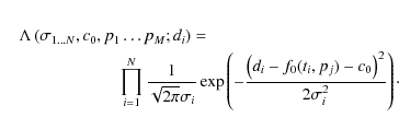
The unknown parameters are denoted by pj, with
First integrating analytically the measurement error ![]() - using Jeffreys'
- using Jeffreys' ![]() -prior - and then the uninteresting offset c0, one gets a likelihood depending only on the spot modelling parameters
-prior - and then the uninteresting offset c0, one gets a likelihood depending only on the spot modelling parameters
![]() .
It is this mean
likelihood, averaged appropriately over measurement error and offset,
from which the posterior density distributions for all unknowns is
obtained by marginalization. This is a great advantage of the Bayesian
approach: it provides not only a set of most probable parameter
values but moreover expectation
values and error bars exclusively from the data. We can argue that the
method itself determines error and offset from the data.
.
It is this mean
likelihood, averaged appropriately over measurement error and offset,
from which the posterior density distributions for all unknowns is
obtained by marginalization. This is a great advantage of the Bayesian
approach: it provides not only a set of most probable parameter
values but moreover expectation
values and error bars exclusively from the data. We can argue that the
method itself determines error and offset from the data.
The Markov chain Monte Carlo (MCMC) method (cf. Press et al. 2007) has been applied to explore the likelihood mountain in a high-dimensional parameter space. The MCMC technique has already shown its capabilities when analysing photometric data from the Canadian MOST satellite (Croll 2006; Fröhlich 2007).
A set of 64 Markov chains was generated. Each chain has to perform some 107 steps, and after a burn-in period every thousandth successful step was recorded in order to suppress the correlation between successive steps. Budding's star-spot model (1977) was used to model the light curve.
Table 4: Spot parameters.
4.1 Results from Bayesian PI
There are two solutions which fit the light curve equally well: one with three ``dark'' spots and another one with four ``bright'' spots. In both cases the residuals amount to 0.12 mmag. The autocorrelation function of the residuals reveals that there is even more in the data than what can be represented by a simple model with circular spots. From a formal point of view the solution with ``dark'' spots is the more probable one, because the fit needs only three spots instead of four. But in view of the spectroscopic evidence the four-spot solution makes much more sense.
The expectation values with 1-![]() confidence limits for the star and the starspot parameters are presented in Table 4. From spot longitudes, spot epochs (HJD) can be computed:
confidence limits for the star and the starspot parameters are presented in Table 4. From spot longitudes, spot epochs (HJD) can be computed:
![]() .
.
The reader should be aware that the estimated parameter values and their (surprisingly small) error bars are those of the model constrained by the data. They make sense given the model is true, i.e. that there are four circular spots, a linear limb-darkening law with prescribed coefficient holds and so forth.
In a further run the coefficient u of the
limb-darkening law has been determined from the data itself. This does
not lead to any improvement of the fit. The fact that the deduced
limb-darkening coefficient
![]() proves to be only a little bit smaller than the
theoretical value of 0.4415 strengthens the confidence in the reliability of the four-spot model.
proves to be only a little bit smaller than the
theoretical value of 0.4415 strengthens the confidence in the reliability of the four-spot model.
The high accuracy of the photometric data makes it reasonable to
question the common wisdom and look for spot evolution as well as
differential rotation and even for a period drift in an Ap star.
Time evolution is described by a Legendre expansion of the logarithm of
the spot areas up to the seventh power in time. We have done this in
the case of the three dark spots only. The result is a clear null
result: we neither find a spot area evolution above a 2.5-![]() level nor a hint for any departure from rigid rotation. The spot periods are constant at
level nor a hint for any departure from rigid rotation. The spot periods are constant at ![]() 3 ppm. The lapping time for the two largest (``dark'') spots would have to exceed 100 years.
3 ppm. The lapping time for the two largest (``dark'') spots would have to exceed 100 years.
It is important to clean the data from a CoRoT orbit effect: the residuals drop by a factor of five by subtracting a periodic signal containing CoRoT's orbital period as well as three overtones (Table 5).
Table 5: CoRoT orbit effect.
| Figure 4: Locations of the four bright photometric spots, assumed to be of circular shape, plotted at five equidistant phases. |
|
| Open with DEXTER | |
5 Magnetic field geometry
All 19 Stokes V LSD-line-profiles derived from ESPaDOnS, NARVAL, and SemelPol spectropolarimetric observations are grouped in a single time-series, in order to increase the rotational sampling as much as possible and build a proper data set for tomographic inversion. The time-series is then used to reconstruct the surface magnetic geometry of the star by means of Magnetic Doppler imaging (Donati & Brown 1997).
![\begin{figure}
\par\includegraphics[width=5.5cm,clip]{12239fg5.eps}
\end{figure}](/articles/aa/full_html/2010/01/aa12239-09/img83.png)
|
Figure 5: Stokes V profiles of HD 50773 after the correction of the mean radial velocity of the star. Black lines represent the data and red/grey lines correspond to the synthetic profiles of our magnetic model. Successive profiles are shifted vertically for better visibility. Rotation phases of observations are indicated in the right part of the plot, and error bars are illustrated on the left of each profile. |
| Open with DEXTER | |
![\begin{figure}
\par\includegraphics[width=9cm,clip]{12239fg6.eps}
\end{figure}](/articles/aa/full_html/2010/01/aa12239-09/img84.png)
|
Figure 6: Magnetic map of HD 50773, reconstructed from Magnetic Doppler imaging. Each chart illustrates the field projection onto one axis of the spherical coordinate frame with, from top to bottom, the radial, azimuthal and meridional field components. The magnetic field strength is expressed in Gauss, and the rotational phases of the observation are indicated as vertical ticks at the top of each chart. |
| Open with DEXTER | |
To compute synthetic Stokes V line profiles, we make a model
of a spherical stellar surface divided into a grid of pixels, each
pixel producing a local Stokes I and V profile.
Assuming a given magnetic field strength and orientation for each
pixel, local Stokes V profiles are calculated under the
assumption, valid in the weak field limit, that Stokes V is proportional to
![]() ,
where
,
where ![]() is the average wavelength of the LSD profile (about 534 nm for HD 50773),
is the average wavelength of the LSD profile (about 534 nm for HD 50773),
![]() is the line-of-sight projection of the local magnetic field vector, g is the effective Landé factor of the LSD profile (equal to 1.2) and
is the line-of-sight projection of the local magnetic field vector, g is the effective Landé factor of the LSD profile (equal to 1.2) and
![]() the wavelength derivative of the local Stokes I
line profile. We further assume that there are no large-scale
brightness or abundance inhomogeneities over the stellar surface,
so that synthetic Stokes I profiles are locally the
same over the whole photosphere. However we would like to mention that
some features in the Stokes V profile variability may arise
from the influence of chemical spots and not from the magnetic topology
itself, which has been demonstrated in Kochukhov et al. (2002).
the wavelength derivative of the local Stokes I
line profile. We further assume that there are no large-scale
brightness or abundance inhomogeneities over the stellar surface,
so that synthetic Stokes I profiles are locally the
same over the whole photosphere. However we would like to mention that
some features in the Stokes V profile variability may arise
from the influence of chemical spots and not from the magnetic topology
itself, which has been demonstrated in Kochukhov et al. (2002).
For each pixel, we impose a Gaussian shape to the local synthetic Stokes I line profile. Parameters of the local profile (width and depth) are chosen to optimise the adjustment of Stokes I
LSD profiles of HD 50773. The amplitude of the local Stokes
profiles for pixels located at the visible hemisphere of the star is
then weighted according to a linear limb-darkening coefficient equal
to 0.49, and their central wavelengths are shifted according to
the line-of-sight velocities of individual pixels, assuming ![]() = 46.3 km s-1 (a value minimising the
= 46.3 km s-1 (a value minimising the ![]() of the magnetic model) and i=40
of the magnetic model) and i=40![]() .
.
Synthetic Stokes V profiles are computed for the
19 observed rotation phases and are compared to the observations.
The data adjustment is iterative and based on a maximum entropy
algorithm (Skilling & Bryan 1984). The version of the code used
here makes a projection of the surface magnetic field onto a spherical
harmonics frame (Donati et al. 2006),
with the magnetic field geometry splitted between a poloidal and
toroidal component (Chandrasekhar 1961). We limit the spherical
harmonics expansion to ![]() .
Using this procedure, the spectropolarimetric data are adjusted at a reduced
.
Using this procedure, the spectropolarimetric data are adjusted at a reduced
![]() (Fig. 5). The final
(Fig. 5). The final ![]() ,
as well as the
reconstructed magnetic topology, are left essentially unchanged as long as the adopted spherical
harmonics description respects
,
as well as the
reconstructed magnetic topology, are left essentially unchanged as long as the adopted spherical
harmonics description respects
![]() .
The reconstructed magnetic geometry is
illustrated in Fig. 6, from which we can easily see that the surface magnetic field
of HD 50773 is mostly a highly inclined dipole, with a polar strength of about 2 kG.
.
The reconstructed magnetic geometry is
illustrated in Fig. 6, from which we can easily see that the surface magnetic field
of HD 50773 is mostly a highly inclined dipole, with a polar strength of about 2 kG.
Table 6: Table of elements and spectral lines used for mapping of HD 50773.
A closer look at the weight of the complex spherical harmonics coefficients
![]() ,
,
![]() ,
and
,
and
![]() (defined by Donati et al. 2006)
is however necessary to obtain a more quantitative information on the
magnetic field distribution. Whereas the inversion procedure allows for
the reconstruction of both poloidal and toroidal components of the
field, 96% of the reconstructed magnetic energy ends up in the
poloidal component. As expected for such a marginal amount of
toroidal field, the outcome of the inversion code is actually almost
similar if we impose the more restrictive case of a purely poloidal
field. As can be readily seen on the map, most of the magnetic
energy (91%) is stored in the dipolar component. Higher-order
field components are however necessary to obtain a convincing
modelling of the observations (up to
(defined by Donati et al. 2006)
is however necessary to obtain a more quantitative information on the
magnetic field distribution. Whereas the inversion procedure allows for
the reconstruction of both poloidal and toroidal components of the
field, 96% of the reconstructed magnetic energy ends up in the
poloidal component. As expected for such a marginal amount of
toroidal field, the outcome of the inversion code is actually almost
similar if we impose the more restrictive case of a purely poloidal
field. As can be readily seen on the map, most of the magnetic
energy (91%) is stored in the dipolar component. Higher-order
field components are however necessary to obtain a convincing
modelling of the observations (up to ![]() ).
Finally, the predominance of a highly non-axisymmetric field
distribution translates into a low amount of magnetic energy in
axis-symmetric spherical harmonics modes (m = 0), which do not gather more than 2% of the overall photospheric magnetic energy.
).
Finally, the predominance of a highly non-axisymmetric field
distribution translates into a low amount of magnetic energy in
axis-symmetric spherical harmonics modes (m = 0), which do not gather more than 2% of the overall photospheric magnetic energy.
6 Spectroscopic Doppler imaging
By applying the Doppler imaging technique (DI), we are
able to translate the partially very pronounced variations in the
spectral line profiles of HD 50773, linked to stellar
rotation, into surface maps of the abundance distribution. The
longitude of a spot is directly deduced from the wavelength position of
the distortion within the profile, whereas its latitude can only be
derived from time-series observations. In the case
of HD 50773, 19 such spectra (listed in Table 1) could be used for the inversions with INVERS12, the DI code we used (Kochukhov et al. 2004b).
In this code, where specific intensities are calculated for each
visible surface element for each iteration, it is possible to
simultaneously calculate abundance maps of several chemical elements
even from blended spectral lines. Mapping HD 50773, we could
derive surface abundance distributions for Mg, Si, Ca, Ti, Cr, Fe, Ni,
Y and Cu. We have to mention that Ti and Ni were derived from
spectral line blends where these elements contribute only moderately to
the overall absorption. Input parameters were determined as described
in Sect. 3,
![]() and inclination i used as in Sect. 5.
and inclination i used as in Sect. 5.
6.1 Surface abundance structures of individual elements
![\begin{figure}
\par\includegraphics[trim = 13.0mm 34mm 8mm 30mm, clip, width=125...
....ps}\\
\includegraphics[width=130mm]{12239fe7.ps}
\vspace*{2.9mm}
\end{figure}](/articles/aa/full_html/2010/01/aa12239-09/img101.png)
|
Figure 7:
Top panel: radial field component of the magnetic map of HD 50773 (as described in Sect. 5). Second panel:
locations of the four bright photometric spots, assumed to be of
circular shape. Next three panels: abundance distribution of Cr, Fe,
and Si at the surface of HD 50773 obtained from the lines listed
in
Table 6.
We show the star at an inclination i = 40 |
| Open with DEXTER | |
![\begin{figure}
\par\includegraphics[width=13.8cm,clip]{12239fa8.ps}\vspace*{-2mm...
...ps}\vspace*{-2mm}
\includegraphics[width=13.8cm,clip]{12239ff8.ps}
\end{figure}](/articles/aa/full_html/2010/01/aa12239-09/img102.png)
|
Figure 8: Same as the three bottom panels in Fig. 7 but for Mg, Ca, Ti, Ni, Y, and Cu. |
| Open with DEXTER | |
6.1.1 Magnesium and calcium
The surface abundance distribution of magnesium was modeled using a blend of Mg I with Fe I and Y II around 5400 Å. We find a variation between
![]() and -3.3 dex and the element, contrary to the other mapped
species, does not exhibit a clear correlation with the magnetic field
geometry, and is enhanced in a spotted, belt-like structure near
the rotational equator (Fig. 8). The abundance distribution of calcium, variable between
and -3.3 dex and the element, contrary to the other mapped
species, does not exhibit a clear correlation with the magnetic field
geometry, and is enhanced in a spotted, belt-like structure near
the rotational equator (Fig. 8). The abundance distribution of calcium, variable between
![]() and -2.7 dex and determined from Ca I and II blended with Fe I
around 6102 Å and 6456 Å also shows a belt-like structure at
the rotational equator with a pronounced region of overabundance at the
positive magnetic pole.
and -2.7 dex and determined from Ca I and II blended with Fe I
around 6102 Å and 6456 Å also shows a belt-like structure at
the rotational equator with a pronounced region of overabundance at the
positive magnetic pole.
6.1.2 Iron-peak elements
A blend of titanium II with Fe I and Cr II at 5169 Å was used to recover the surface abundance structure of this element. Ti II shows a tendency to accumulate at the magnetic poles and to avoid the magnetic equatorial regions, varying between
![]() and -6.1 dex.
and -6.1 dex.
Chromium was mapped using several single Cr lines at 5237 Å and 5280 Å plus a blend of
Cr II with Fe I Y II and Ni I around 5510 Å and was found to be variable between
![]() and -3.0 dex. The abundance distribution of the element shows
as that of Fe a clear correlation to the magnetic field geometry, being
enhanced at the poles and depleted at the magnetic equator, whereby the
two enhancement regions seem to be subdivided into two spots.
and -3.0 dex. The abundance distribution of the element shows
as that of Fe a clear correlation to the magnetic field geometry, being
enhanced at the poles and depleted at the magnetic equator, whereby the
two enhancement regions seem to be subdivided into two spots.
The surface abundance of iron was determined using single Fe I lines at 5383 Å and 5400 Å and again the blend of Fe I with Cr II, Y II, and Ni I
at 5510 Å. As mentioned above, Fe is, as Cr,
closely correlated with the magnetic field, avoiding the magnetic
eqatorial region. The elemental abundance varies between
![]() and -1.9 dex.
and -1.9 dex.
Nickel, derived from the blend of this element with Cr II, Fe I, and Y II at 5510 Å and variable between
![]() and -5.6 dex shows an opposite correlation to the magnetic field
geometry from what we saw from Cr and Fe: it is enhanced
at the magnetic equatorial regions and depleted where the positive and
the negative magnetic pole cross the line of sight.
and -5.6 dex shows an opposite correlation to the magnetic field
geometry from what we saw from Cr and Fe: it is enhanced
at the magnetic equatorial regions and depleted where the positive and
the negative magnetic pole cross the line of sight.
6.1.3 Yttrium and copper
A similar distribution as that for Ni can be observed for yttrium. Varying from
![]() to
-7.7 dex it also shows a pronounced region of overabundance at the
magnetic equator and depletion on the poles. The element was mapped
from a blend with Cr II, Fe I, and Ni I at 5510 Å and 5662 Å. Copper around 5153 Å, blended with Cr II, Ti II, and Fe I was used to derive the surface abundance of this element, and we see it to vary between
to
-7.7 dex it also shows a pronounced region of overabundance at the
magnetic equator and depletion on the poles. The element was mapped
from a blend with Cr II, Fe I, and Ni I at 5510 Å and 5662 Å. Copper around 5153 Å, blended with Cr II, Ti II, and Fe I was used to derive the surface abundance of this element, and we see it to vary between
![]() and -6.9 dex. At first glance, it seems to be closely
related to the distributions of Ni and Y, being enhanced at
the magnetic equator, but it exhibits in addition two less pronounced
spots close to the magnetic poles.
and -6.9 dex. At first glance, it seems to be closely
related to the distributions of Ni and Y, being enhanced at
the magnetic equator, but it exhibits in addition two less pronounced
spots close to the magnetic poles.
7 Effect of abundance inhomogeneities on spectral energy distribution
As already mentioned in Sect. 1
the light curve of HD 50773 obtained by CoRoT has a periodic form
with two clear maxima of slightly different atmplitudes at phases ![]()
![]() 0.05 and 0.52 (see Fig. 1).
This photometric variability is likely to be connected with
inhomogeneous surface element distributions, similar to those recently
reported and successfully modeled by Krticka et al. (2007)
for the hot CP2 star HD 37776. The physical nature of this effect
is directly connected with the radiative flux redistribution due to
enhanced or deficient opacity in the abundance spots relative to the
rest of the stellar surface. Hence, as a star rotates, the
observer sees different stellar regions that are emitting a different
amount of radiative flux producing characteristic variability of
indices in phase-resolved photometry.
0.05 and 0.52 (see Fig. 1).
This photometric variability is likely to be connected with
inhomogeneous surface element distributions, similar to those recently
reported and successfully modeled by Krticka et al. (2007)
for the hot CP2 star HD 37776. The physical nature of this effect
is directly connected with the radiative flux redistribution due to
enhanced or deficient opacity in the abundance spots relative to the
rest of the stellar surface. Hence, as a star rotates, the
observer sees different stellar regions that are emitting a different
amount of radiative flux producing characteristic variability of
indices in phase-resolved photometry.
Of course, abundance spots are not the only effect which may produce visible rotational modulation in photometry. For instance, strong magnetic fields may also influence the total radiative flux gradients along the stellar surface since the magnetic opacity and flux distribution strongly depend upon the modulus of the magnetic field (Kochukhov et al. 2005; Khan & Shulyak 2006). However, the mean surface magnetic field of HD 50773 is too weak to noticeably affect the integrated opacity coefficient, and thus the chemical spots are the most probable source of the observed variability. Details of our modelling of the light variability taking into account surface abundance variations of HD 50773 are presented in this section.
Having produced abundance maps using the Doppler imaging technique it is, in principle, possible to directly model the light curve variability in the same manner as it was done in Krticka et al. (2007). However, in case of HD 50773, there are several elements that play a noticeable role in the flux redistribution, which would require the calculation of hundreds of model atmospheres for an accurate surface integration. These extensive computations are out of the scope of the present paper. Nevertheless, to explore the role of the mapped elements on the total energy balance in the atmosphere of HD 50773 (and thus on the ability of these elements to affect the radiative balance) we computed a set of model atmospheres with different assumptions about abundance patterns. To carry out such calculations we employed the LL MODELS stellar model atmosphere code (Shulyak et al. 2004), which incorporates treatment of individual abundance patterns and computes the line opacity in a fine frequency grid for better integration of the radiation field quantities.
First we computed the model with the surface averaged abundances of all nine elements used in our DI analysis. Then another seven models were computed, individually increasing every element by +2 dex relative to its mean value. Once these computations were done, we integrated the output radiative fluxes from all the models and then compared them to the flux produced by the mean abundance reference model. The flux integration was performed in the wavelength range defined by the CoRoT photometric CCD, i.e. from 2500 Å to 11 000 Å, with the resolution of 0.1 Å, which is the default flux resolution in LL MODELS. The effective temperature of all the models was kept to be the same.
We find that among the nine elements considered in this investigation only four have a clear influence on the model energy distribution by more than 1%. These elements are Cr (1.16%), Fe (5.63%), Mg (3.02%), and Si (2.21%). The influence of the other five elements is much less pronounced like, e.g. Ca (0.22%). This agrees well with the recent study of Khan & Shulyak (2007) who investigated the effect of individual chemistry on properties of CP stars and showed the relative importance of Fe, Cr, and Si opacity for all the models considered.
As an example, Fig. 9 demonstrates the synthetic energy distribution computed with enhanced abundances of Cr, Fe, Mg, and Si. In particular, one can note the strong impact of Fe and Si on the shape of the energy distribution. However, the relatively small changes in integrated flux values listed above are due to the fact that the CoRoT photometry covers a wide wavelength region where the flux changes due to enhanced abundance models which act in opposite directions in the UV and the visual regime. We do not show fluxes produced by the other mapped elements since they lie extremely close to the flux of the mean abundance model (thick full line).
![\begin{figure}
\par\includegraphics[angle=-90,width=16.8cm,clip]{12239fg9.eps}
\end{figure}](/articles/aa/full_html/2010/01/aa12239-09/img112.png)
|
Figure 9: The synthetic energy
distributions of HD 50773 calculated with mean surface abundances
and abundances of Cr, Fe, Mg, and Si enhanced by 2 dex. For
all models
|
| Open with DEXTER | |
8 Conclusions
The high-quality CoRoT data enabled us by applying the Bayesian data analysis to derive stellar surface structures from space quality photometry. Analysing an extensive set of ground based spectropolarimetric data via Doppler imaging and Magnetic Doppler imaging made it possible to directly correlate the results from photometry to the chemical and magnetic stellar surface structure. The resulting abundances were used to model the light variability of HD 50773.
The two areas covered by bright spots found with Bayesian data analysis of the light curve coincide very well with the magnetic polar regions on the surface of HD 50773.
The elemental abundance spots of the species contributing dominantly to the changes in the integrated flux (Cr, Fe, and Si) are also clearly correlated with the magnetic field geometry and hence with photometric spots. Regions of overabundance are found close to the magnetic poles and those of depletion linked to the magnetic equator. As described in Sect. 7, these elements produce bright spots in the photosphere.
Our results confirm the high potential of combining high quality photometric data obtained in space with ground based spectroscopy. Further studies with a similar approach are currently ongoing and will significantly increase the sample of stars analysed in this way, which is important for modelling elemental diffusion in stars in the presence of a magnetic field.
AcknowledgementsWe would like to thank the referee, Z. Mikulásek, for very consctructive comments during the refereeing process. We also thank the CoRoT, CFHT and TBL teams for their observing support and the excellent data, and N. Letourneur and J.-P. Michel, who obtained the NARVAL spectra for us. This work was supported by the Austrian Science Fund FWF-P17580N2, the Lise Meitner grant No. M998-N16 to DS and by the financial contributions of the Austrian Agency for International Cooperation in Education and Research (WTZ CZ-11/2008). O.K. is a Royal Swedish Academy of Sciences Research Fellow supported by a grant from the Knut and Alice Wallenberg Foundation.
References
- Asplund, M., Grevesse, N., & Sauval, A. J. 2005, ASP Conf. Ser., 336, 25 [Google Scholar]
- Appourchaux, T., Michel, E., Auvergne, M., et al. 2008, A&A, 488, 705 [Google Scholar]
- Auvergne, M., Bodin, P., Boisnard, L., et al. 2009, A&A, 506, 411 [Google Scholar]
- Baglin, A., Michel, E., Auvergne, M., et al. 2006, in ESA SP, 1306, 3950 [Google Scholar]
- Babel, J. 1992, A&A, 258, 449 [Google Scholar]
- Boisnard, L., & Auvergne, M. 2006, Proceedings of The CoRoT Mission Pre-Launch Status - Stellar Seismology and Planet Finding, ed. M. Fridlund, A. Baglin, J. Lochard, & L. Conroy, ESA SP-1306, 19 [Google Scholar]
- Budding, E. 1977, Ap&SS, 48, 207 [Google Scholar]
- Croll, B. 2006, PASP, 118, 1351 [NASA ADS] [CrossRef] [Google Scholar]
- Donati, J.-F., Semel, M., Carter, B. D., et al. 1997, MNRAS, 291, 658 [NASA ADS] [CrossRef] [MathSciNet] [Google Scholar]
- Donati, J.-F., Collier Cameron, A., Hussain, G. A. J., & Semel, M. 1999, MNRAS, 302, 437 [NASA ADS] [CrossRef] [Google Scholar]
- Donati, J.-F., Cameron, A. C., Semel, M., et al. 2003, MNRAS, 345, 1145 [NASA ADS] [CrossRef] [Google Scholar]
- Donati, J.-F., Howarth, I. D., & Jardine, M. M. 2006, MNRAS, 370, 629 [NASA ADS] [CrossRef] [Google Scholar]
- Fridlund, M., Baglin, A., Lochard, J., & Conroy, L. 2006, The CoRoT Mission, ESA SP-1306 [Google Scholar]
- Fröhlich, H.-E. 2007, Astron. Nachr., 328, 1037 [NASA ADS] [CrossRef] [Google Scholar]
- Khan, S. A., & Shulyak, D. V. 2006, A&A, 448, 1153 [Google Scholar]
- Khan, S. A., & Shulyak, D. V. 2007, A&A, 469, 1083 [Google Scholar]
- Kochukhov, O. 2007, Physics of Magnetic Stars, ed. I. I. Romanyuk, & D. O. Kudryavtsev, 109 [Google Scholar]
- Kochukhov, O., & Piskunov, N. 2002, A&A, 388, 868 [Google Scholar]
- Kochukhov, O., Drake, N. A., Piskunov, N., & de la Reza, R. 2004, A&A, 424, 935 [Google Scholar]
- Kochukhov, O., Khan, S., & Shulyak, D. 2005, A&A, 433, 671 [Google Scholar]
- Krticka, J., Mikulásek, Z., Zverko, J., & Zizåovský, J. 2007, A&A, 470, 1089 [Google Scholar]
- Krticka, J., Mikulásek, Z., Henry, G. W., et al. 2009, A&A, 499, 56 [Google Scholar]
- Kupka, F., Piskunov, N., Ryabchikova, T. A., Stempels, H. C., & Weiss, W. W. 1999, A&AS, 138, 119 [Google Scholar]
- Kurucz, R. L. 1993, Kurucz CD-ROM, Cambridge, MA, Smithsonian Astrophysical Observatory, December 4, sssp.book [Google Scholar]
- Mikulásek, Z., Krticka, J., Zverko, J., et al. 2007, in Physics of Magnetic Stars, ed. I. I. Romanyuk, & D. O. Kudryavtsev, Special Astrophys. Obs., Nizhnij Arkhyz, 300 [Google Scholar]
- Mikulásek, Z., Gráf, T., Krticka, J., Zverko, J., & Ziznovský, J. 2008a, Contr. Astron. Obs. Sk. Pleso, 38, 363 [Google Scholar]
- Mikulásek, Z., Krticka, J., Henry, G. W., Zverko, J., & Zizåovský, J. 2008b, A&A, 485, 585 [Google Scholar]
- Michaud, G. 1970, ApJ, 160, 640 [Google Scholar]
- Piskunov, N. E., Kupka, F., Ryabchikova, T. A., Weiss, W. W., & Jeffery, C. S. 1995, A&AS, 112, 525 [Google Scholar]
- Press, W. H., Teukolsky, S. A., Vetterling, W. T., & Flannery, B. P. 2007, Numerical Recipes, 3rd edn (Cambridge: Cambridge Univ. Press) [Google Scholar]
- Renson, P., Gerbaldi, M., & Catalano, F. A. 1991, A&AS, 89, 429 [Google Scholar]
- Ryabchikova, T. A., Piskunov, N. E., Stempels, H. C., Kupka, F., & Weiss, W. W. 1999, Phys. Scr, T83, 162 [Google Scholar]
- Rees, D. E., & Semel, M. 1979, A&A, 74, 1 [Google Scholar]
- Semel, M., Donati, J.-F., & Rees, D. E. 1993, A&A, 278, 231 [Google Scholar]
- Shulyak, D., Tsymbal, V., Ryabchikova, T., Stütz, Ch., & Weiss, W. W. 2004, A&A, 428, 993 [Google Scholar]
- Stibbs, D. W. N. 1950, MNRAS, 110, 410 [Google Scholar]
Footnotes
- ... HD 50773
- The CoRoT space mission was developed and is operated by the French space agency CNES, with participation of ESA's RSSD and Science Pograms, Austria, Belgium, Brazil, Germany, and Spain.
All Tables
Table 1:
Journal of the spectroscopic observations of HD 50773: dates, instrument, exposure time, peak S/N, HJD, phase, ![]() ,
, ![]() .
.
Table 2: Abundances of 17 species derived from equivalent width measurements in co-added spectra of HD 50773.
Table 3: Line list used for abundance analysis based on equivalent width measurements in the co-added spectrum of HD 50773.
Table 4: Spot parameters.
Table 5: CoRoT orbit effect.
Table 6: Table of elements and spectral lines used for mapping of HD 50773.
All Figures
|
|
Figure 1: Phase plot of HD 50773 using a binned light curve after the subtraction of effects due to the CoRoT orbit and the stellar signal not attributed to rotation. Overplotted (white line) is the four-spot model fit described in Sect. 4 of this paper. |
| Open with DEXTER | |
| In the text | |
|
|
Figure 2: Upper panel: the CoRoT light curve of HD 50773 after removal of the obvious stellar variability (black). Some small flux changes are remaining, which are shown in grey after applying a running average (see text in this section). Lower panel: after the subtraction of this running average, the residuals to the stellar variability are mostly consistent with white noise. Note that the abscissa in this plot is in CoRoT - HJD (=HJD-2 451 545.0) and the ordinate in CoRoT - internal flux units of the N2 data level after subtraction of the mean photometric signal, which is 301 700 in the same units. |
| Open with DEXTER | |
| In the text | |
|
|
Figure 3: Upper panel: the detrended CoRoT light curve of HD 50773 and the resampled running average containing information about residual signal obviously not related to stellar rotation (thick black line). Lower panel: the final light curve containing only signal due to stellar rotation and used for the Bayesian analysis, but zero-mean corrected for the sake of comparability. Again the abscissa in this plot is in CoRoT - HJD (=HJD-2 451 545.0) and the ordinate in CoRoT - internal flux units of the N2 data level after subtraction of the mean photometric signal, which is 301 700 in the same units. |
| Open with DEXTER | |
| In the text | |
| |
Figure 4: Locations of the four bright photometric spots, assumed to be of circular shape, plotted at five equidistant phases. |
| Open with DEXTER | |
| In the text | |
|
|
Figure 5: Stokes V profiles of HD 50773 after the correction of the mean radial velocity of the star. Black lines represent the data and red/grey lines correspond to the synthetic profiles of our magnetic model. Successive profiles are shifted vertically for better visibility. Rotation phases of observations are indicated in the right part of the plot, and error bars are illustrated on the left of each profile. |
| Open with DEXTER | |
| In the text | |
|
|
Figure 6: Magnetic map of HD 50773, reconstructed from Magnetic Doppler imaging. Each chart illustrates the field projection onto one axis of the spherical coordinate frame with, from top to bottom, the radial, azimuthal and meridional field components. The magnetic field strength is expressed in Gauss, and the rotational phases of the observation are indicated as vertical ticks at the top of each chart. |
| Open with DEXTER | |
| In the text | |
|
|
Figure 7:
Top panel: radial field component of the magnetic map of HD 50773 (as described in Sect. 5). Second panel:
locations of the four bright photometric spots, assumed to be of
circular shape. Next three panels: abundance distribution of Cr, Fe,
and Si at the surface of HD 50773 obtained from the lines listed
in
Table 6.
We show the star at an inclination i = 40 |
| Open with DEXTER | |
| In the text | |
|
|
Figure 8: Same as the three bottom panels in Fig. 7 but for Mg, Ca, Ti, Ni, Y, and Cu. |
| Open with DEXTER | |
| In the text | |
|
|
Figure 9: The synthetic energy
distributions of HD 50773 calculated with mean surface abundances
and abundances of Cr, Fe, Mg, and Si enhanced by 2 dex. For
all models
|
| Open with DEXTER | |
| In the text | |
Copyright ESO 2010
Current usage metrics show cumulative count of Article Views (full-text article views including HTML views, PDF and ePub downloads, according to the available data) and Abstracts Views on Vision4Press platform.
Data correspond to usage on the plateform after 2015. The current usage metrics is available 48-96 hours after online publication and is updated daily on week days.
Initial download of the metrics may take a while.