---

Non-linear evolution of the diocotron instability in a pulsar electrosphere: two-dimensional particle-in-cell simulations

J. Pétri¹

Observatoire Astronomique de Strasbourg, 11 rue de l'Université, 67000 Strasbourg, France

Received 3 February 2009 / Accepted 27 April 2009

Abstract
Context. The physics of the pulsar magnetosphere near the neutron star surface remains poorly constrained by observations. Indeed, little is known about its emission mechanism, from radio to high-energy X-ray and gamma-rays. Nevertheless, it is believed that large vacuum gaps exist in this magnetosphere, and a non-neutral plasma partially fills the neutron star surroundings to form an electrosphere in differential rotation.
Aims. According to several of our previous works, the equatorial disk in this electrosphere is diocotron and magnetron unstable, at least in the linear regime. To better assess the long term evolution of these instabilities, we study the behavior of the non-neutral plasma using particle simulations.
Methods. We designed a two-dimensional electrostatic particle-in-cell (PIC) code in cylindrical coordinates, solving Poisson equation for the electric potential. In the diocotron regime, the equation of motion for particles obeys the electric drift approximation. As in the linear study, the plasma is confined between two conducting walls. Moreover, in order to simulate a pair cascade in the gaps, we add a source term feeding the plasma with charged particles having the same sign as those already present in the electrosphere.
Results. First we checked our code by looking for the linear development of the diocotron instability in the same regime as the one used in our previous work, for a plasma annulus and for a typical electrosphere with differential rotation. To very good accuracy, we retrieve the same growth rates, supporting the correctness of our PIC code. Next, we consider the long term non-linear evolution of the diocotron instability. We found that particles tend to cluster together to form a small vortex of high charge density rotating around the axis of the cylinder with only little radial excursion of the particles. This grouping of particles generates new low density or even vacuum gaps in the plasma column. Finally, in more general initial configurations, we show that particle injection into the plasma can drastically increase the diffusion of particles across the magnetic field lines. The newly formed vacuum gaps cannot be replenished by simply invoking diocotron instability.
Conclusions. Diocotron instability offers a new possibility to solve the current closure problem in a pulsar magnetosphere. It is a promising mechanism leading to highly unstable flows in the pulsar inner magnetosphere. When flowing towards the light cylinder, some relativistic and particle inertia effects (not included in this study) appear. Nevertheless, the system should remain unstable because of the relativistic diocotron or the magnetron instability. Therefore, we expect an electric current to circulate in the closed magnetosphere and to feed the base of the wind with charged particles.

Key words: instabilities - plasmas - methods: numerical - pulsars: general

1 Introduction

The detailed structure of charge distribution and electric-current circulation in the closed magnetosphere of a pulsar remains puzzling. Although it is often assumed that the plasma fills the space entirely and corotates with the neutron star, it is on the contrary very likely that it only partly fills it, leaving large vacuum gaps between plasma-filled regions. The existence of such gaps in aligned rotators has been very clearly established by Krause-Polstorff & Michel (1985b,a). Since then, a number of different numerical approaches to the problem have confirmed their conclusions, including some work by Rylov (1989), Shibata (1989), Zachariades (1993), Neukirch (1993), Thielheim & Wolfsteller (1994), Spitkovsky & Arons (2002), and ourselves (Pétri et al. 2002b). This conclusion about the existence of vacuum gaps has been reached from a self-consistent solution of the Maxwell equations in the case of the aligned rotator. Moreover, Smith et al. (2001) have shown by numerical modelling that an initially filled magnetosphere like the Goldreich-Julian model evolves by opening up large gaps and stabilizes at the partially filled and partially void solution found by Krause-Polstorff & Michel (1985a) and also by Pétri et al. (2002b). The status of models of the pulsar magnetospheres, or electrospheres, has been critically reviewed by Michel (2005). A solution with vacuum gaps has the peculiar property that those parts of the magnetosphere that are separated from the star's surface by a vacuum region are not corotating and so undergo differential rotation, an essential ingredient that will lead to non-neutral plasma instabilities in the closed magnetosphere.

This kind of non-neutral plasma instability is well known to plasma physicists (O'Neil & Smith 1992; Oneil 1980; Davidson 1990). Their good confinement properties makes them a valuable tool for studying plasmas in the laboratory, by using for instance Penning traps. In the magnetosphere of a pulsar, far from the light cylinder and close to the neutron star surface, the instability reduces to its non-relativistic and electrostatic form, the diocotron instability. The linear development of this instability for a differentially rotating charged disk was studied by Pétri et al. (2002a), in the thin disk limit, and by Pétri (2008,2007a,b) in the thick disk limit. It both cases, the instability proceeds at a growth rate comparable to the star's rotation rate. The non-linear development of this instability was studied by Pétri et al. (2003), in the framework of an infinitely thin disk model. They have shown that the instability causes a cross-field transport of these charges in the equatorial disk, evolving into a net out-flowing flux of charges. Spitkovsky & Arons (2002) have numerically studied the problem and concluded that this charge transport tends to fill the gaps with plasma. The appearance of a cross-field electric current as a result of the diocotron instability has been observed by Pasquini & Fajans (2002) in laboratory experiments in which charged particles were continuously injected in the plasma column trapped in a Malmberg-Penning configuration.

Numerical simulations of the non-linear development of the diocotron instability have been investigated by different authors. For instance, Pétri et al. (2003) used a numerical scheme similar to those used for MHD codes. This has the drawback of poorly treating vacuum gaps which eventually are created in the electrosphere. To better deal with these gaps, we decided to design a particle simulation code that does not suffer from the presence of vacuum. Particle-in-cell (PIC) methods have already been successful in investigating the diocotron instability (Yatsuyanagi et al. 2003; Neu & Morales 1995). Problems with injection have also been considered see for instance Bettega et al. (2007).

In this paper, we extend the work initiated by Pétri (2007b) and look for the non-linear evolution of the diocotron instability by performing 2D electrostatic PIC simulations. The question of the influence of pair creation will also be addressed by permitting injection of charged particles into the system. The paper is organized as follows. In Sect. 2, we briefly recall the initial setup of the plasma column as done in Pétri (2007b). In Sect. 3, we show the results of our 2D PIC simulations. First we checked the code by computing some linear growth rates for special cases like a constant density plasma column for which we know exact analytical solutions, see for instance Pétri (2007a). Second, we check that we retrieve the same linear growth rates for the electrosphere as those found in Pétri (2007b). Third, we let the system evolve on long time scales and look for significant particle diffusion. Finally, in a last set of runs, we injected some charged particles into the system to study the behavior of the instability in the presence of a source of charges, Sect. 4. The extreme case starting with vacuum will also be presented. The conclusions and the possible generalizations are presented in Sect. 5.

2 The model

We first review the plasma configuration as described in Pétri (2007b). We study the motion of a non-neutral plasma column of infinite axial extend along the z-axis. We adopt cylindrical coordinates denoted by  and define the corresponding orthonormal basis vectors by  . In the initial state corresponding to an equilibrium, the plasma is only rotating in the azimuthal direction, with no motion in the radial direction along ror the vertical direction along z.

2.1 Plasma and field setup

Unlike other magnetospheric models, our pulsar electrospheric plasma is assumed to be completely charge-separated. So we consider a single-species non-neutral fluid consisting of particles with mass  and charge q trapped between two cylindrically conducting walls located at the radii W₁ and W₂ > W₁. The plasma column itself is confined between the radii and , with R₁<R₂. This allows us to take into account vacuum regions between the plasma and the conducting walls. Such geometric configurations will also be useful to investigate particle diffusion across magnetic field lines into this vacuum and will clearly demonstrate the efficiency of the diocotron instability to fill gaps with plasma, as shown in some examples in the last section.

In order to simulate the presence of a charged neutron star generating a radial electric quadrupole field coming from the rotating magnetic dipole, the inner wall at W₁ can carry a charge Q per unit length such that its electric field is simply given by the Maxwell-Gauss theorem, (we use MKSA units)

In the equilibrium configuration, the particle number density is n(r) and the charge density is  . In contrast to earlier studies, the external magnetic field, along the z-axis, is not necessarily uniform but can decrease with radius

The electric field is made of two parts, the first one arising from the plasma column  itself, and the second one from the inner conducting wall  , Eq. (1). We assume that the electric field induced by the plasma vanishes at r=W₁, i.e. . Applying the Maxwell-Gauss equation, we solve for the equilibrium electric field and get

The total electric field, directed along the radial direction,  , is therefore the sum

In the non-relativistic diocotron regime, we do not solve the full set of Maxwell equations but only the electrostatic part. This means that the magnetic field perturbation induced by the plasma flow is neglected. Thus, the externally imposed magnetic field, Eq. (2), remains constant during the simulations. This assumption is justified when the plasma is confined well inside the light-cylinder and when its rest mass energy density remains negligible compared to the magnetic field energy density, in other words

with c the speed of light in vacuum.

2.2 Equation of motion

The motion of the plasma is governed by the conservation of charge, which in the non-neutral plasma case is equivalent to conservation of the number of particles, the Maxwell-Poisson equation, and the electric drift approximation, respectively

is the usual electric potential associated with the total electric field, Eq. (4) (plasma distribution + externally applied electric field). We use the usual notation, for the electric charge density, for the velocity, for the electromagnetic field. The set of Eqs. (6)-(9) fully describes the non-linear time evolution of the cold plasma in the non-relativistic diocotron regime. Note that particle inertia does not enter into the abovementioned expressions. The gyromotion is averaged over the fastest timescale, leading to the electric drift approximation, as long as this drift speed remains lower than the speed of light, in other words, as long as E<c B. In Eqs. (6)-(9), there is no reference to the speed of light because we are in the non-relativistic regime. Formally it corresponds to the limit ; electromagnetic waves propagate instantaneously. Therefore, at this stage, it is impossible to check whether the electric field intensity E remains smaller than c B or not. The hypothesis E<c B is implicitly always true in our model because of the electric drift approximation. Indeed v<c in Eq. (8) implies E<c B. It is an implicit assumption that we presume to be valid during all simulations. To include relativistic effects, we would have to solve the full set of Maxwell equations, as was done to investigate the relativistic stabilization of the diocotron instability in the linear regime, see for instance Pétri (2007a). This would introduce a timescale related to the speed of light c. Performing 2D relativistic PIC simulations of the diocotron instability is the purpose of ongoing work and will be presented in a forthcoming paper.

2.3 Code description

We designed an algorithm using standard techniques for particle in cell (PIC) codes (Birdsall & Langdon 2005; Hockney 1988). We use explicit schemes to advance both the particles and the electric field in time. A description of our own code on how to evolve field and particles is briefly discussed in the following subsections.

2.3.1 Integration of the equation of motion

We assume that the inner and outer conductors act mechanically as solid walls in such a way that particles are reflected at these boundaries. The equation of motion for particles in the electric drift approximation takes a very simple form, allowing us to solve immediately for the velocity vector, see Eq. (8). From a computational point of view, this equation of motion, Eq. (8), is integrated with a leapfrog scheme, which is second order in time. More precisely, denoting as the time at the nth iteration, where is the time step, positions are computed at integer times tⁿ whereas velocities are computed at half-integer times for each particle labelled with the index i such that

The electromagnetic field at half-integer time is evaluated from the position of the particles at the same time, positions updated according to the speed known only at preceding times t^n-1/2:

Then, the electromagnetic field at half-integer time following from these positions at the location of particle number i are

We use a Lagrangian description, which means that no grid is associated with the position of the particle. Because the initial velocity and position are given for t=0 by  and  , we initialize the speed of the particles by first doing half a time step forwards in order to find

We then evolve positions and velocities according to Eqs. (10), (11). Note that in all the simulations, the electric and magnetic fields do not explicitly depend on time.

2.3.2 Field solver

The Poisson equation is solved on an Eulerian grid by a Fourier transform in the azimuthal direction  and a finite difference scheme for the radial dependence. Note that in Eq. (10), both the electric and the magnetic fields are evaluated at a half-integer time t^n+1/2. Because the electric field is derived from a potential , we need only to consider a scalar Poisson equation. The potential  as well as the charge density are developed into a real / Fourier series as

is the number of discretization points in the azimuthal direction. Thus the Poisson equation transforms into a set of ordinary differential equations for the unknown functions as follows

Because of the linearity of the Poisson equation, the azimuthal modes decouple into a set of independent ordinary differential equations for each natural integer m. Using a classical finite difference discretization in radius, we derive a set of matrices for each pair of unknown functions  to be solved by standard linear algebra techniques. However, the structure of the discretization matrices is tridiagonal, allowing to use numerical algorithms that are more efficient, see for instance Press (2002). Moreover, as an outer boundary condition, we ensure a vanishing electric potential at the outer wall which is expressed as , whereas at the inner boundary, we enforce either a vanishing derivative d /dr = 0corresponding to nullifying the normal component of the electric field for the vacuum or plasma annuli cases, or the corotation electric field for the electrosphere, in order to adjust smoothly to the revolution of the compact object (assuming ideal MHD).

Charges are deposited on the Eulerian grid  in order to deduce the source terms  for the Poisson equation. The electromagnetic field is evaluated on particle positions by 2D linear interpolation between points in this Eulerian grid  .

2.3.3 Particle injection

Finally, we simulate the pair creation mechanism in the magnetosphere by injecting charged particles somewhere inside the system. The deposition is uniform in the azimuthal direction and prescribed to be at a given radius and rate, both fixed by the user. Typically, we took an injection radius  . Formally, the shape function can be thought of a delta-Dirac distribution in the radial direction, let us say . is the particle flux. Nevertheless, this is a user-defined source function and can be taken to behave very differently, and can also evolve in space and time. There is no particular restriction on its shape. As a starting point, we took the most simple dependence, constant in time and and sharply concentrated in radius. To be more realistic, pair creation should be incorporated by taking into account different processes like photon-photon disintegration or photon-(strong) magnetic field interaction (which is formally the same process as the former, as the magnetic field can be thought of as a photon field from a quantum mechanical point of view). Monte Carlo simulations would be a valuable tool for such a study, but this will not be included in this work.

3 Results without particle injection

First, we checked our algorithm in different configurations by picking out the linear regime from our runs and compare the growth rates with those predicted by the linear analysis.

In order to keep the particle noise as weak as possible to clearly see the linear stage evolving over a few order of magnitudes, we need to start with an initial state with minimal energy. This is achieved by using a so-called ``quiet start'', such that space is regularly filled with particles, see for instance Birdsall & Langdon (2005).

The resolution of the spatial grid on which the electric potential is solved and charge is deposited is , if not otherwise specified. On average, at the beginning of the runs, there are 25 particles per cell, giving a total number of 1 280 000. Time is given in units of where is the cyclotron frequency. We also tried different resolutions and find no qualitative discrepancy, we adopted the aforementioned canonical values.

Note that for all the runs shown below, the charge Q carried by the inner conductor is set to zero, Q=0. The purpose of this work is not to make a parametric study of the diocotron instability behavior but rather to point out its main non-linear characteristics for a closed (without particle injection or loss) and an open (with particle injection or loss) system. Moreover, in this and subsequent sections, the magnetic field is uniform and constant over the whole plasma column. Let us now discuss the main results.

3.1 Plasma annulus

Table 1:   Eigenvalues  for the constant density plasma annulus, for different modes m and different aspect ratios, d₁ = R₁ / W₂, and d₂ = R₂ / W₂, obtained from the analytical expression found in Davidson (1990).

For completeness, we briefly recall the main characteristics of the configuration. The magnetic field is constant and uniform outside the plasma annulus, namely B_z = B₀, for r>R₂. We solve the Maxwell-Poisson equation in the space between the inner and the outer wall, R₁ < r < R₂. The particle number density and charge density are constant over the whole plasma column such that

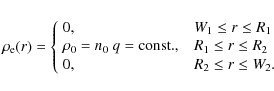
To initiate the instability, we disturb the axisymmetric configuration by overlapping a tiny density perturbation with a relative magnitude (i.e. compared to the background density) of the order h=10^-6. To pick out a given mode, the perturbation is modulated with the appropriate azimuthal pattern m. To be more precise, the initial axisymmetric equilibrium position of each particle is perturbed according to

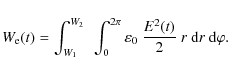
In this cylindrical geometry, an exact analytical solution of the dispersion relation has been found for the diocotron instability, see Davidson (1990). We use these results to check our code, as was already done in Pétri (2007a). Some exact analytical eigenvalues are listed in Table 1 for different radial plasma extensions and azimuthal modes. In order to quantify the growth rate of the diocotron instability in our simulations, we estimate the total electrostatic energy in the system by computing the integral

To determine the linear growth phase, we calculate the increase in electrostatic energy by determining the difference between the actual and the initial electrostatic energy as

Note that because is a quadratic expression with respect to the perturbed quantities, the linear growth rate for the electrostatic energy increase will be twice the value given in Table 1.

Two examples of a run are now discussed. The simulation domain is located between W₁=1 and W₂=10. For the first run, the plasma annulus is located between R₁=4 and R₂=5 with a perturbation m=3, called A1, while for the second run we took R₁=6, R₂=7with a perturbation m=7, called A2. We examine the evolution of the electrostatic energy given by Eq. (23) and depicted in Fig. 1 on a logarithmic scale.

For the first run, at small times, t<100, the linear regime sets in and the measured growth rate is close to the one predicted by linear analysis (red straight line); the perturbed pattern grows at a speed predicted by the linear theory. The plasma column stays roughly confined between R₁ and R₂ and no strong density rearrangement is perceptible. Note also that no other mode is excited and no cascade due to non-linear effects is observed because they are to weak.

In some runs, such as the first mentioned above, it can happen that the initial electrostatic fluctuations decrease slightly before a significant increase of many orders of magnitude, after a while, inducing a  at the beginning and thus making the logarithm not defined at this early stage. In Fig. 1, it is unreliable to give a physical interpretation to this initial behaviour because it corresponds to numerical round off error, close to the machine precision (we work with double precision numbers, i.e. 16 significant digits). Moreover, the gaps are probably due to the particle noise inherent in the PIC method, proportional to the inverse of the square root of the number of particles N, (i.e. N^-1/2). Tiny fluctuations in positions, especially particles receding to the inner wall, tend to decrease the total electrostatic energy, at least at the beginning of the simulations.

In a second step, non-linear effects come into play and the initial plasma distribution is destroyed. The azimuthal pattern with the typical m=3 mode becomes clearly visible in left part of Fig. 2. Particles ``merge'' to form large vortices and leave behind them vacuum gaps which will not be replenished. For some time, these vortices rotate around the axis of the cylinder, keeping their m=3 structure. In a last step, almost all particles hit the inner wall W₁; this happens when t>400. The total electrostatic energy saturates, reaching a plateau at the end. When the non-linear effects set in, we are interested in the diffusion of particles across magnetic field lines and on its consequences on a longer timescale. To get a better idea of this diffusion process, we quantify it by computing the azimuthally integrated charge density as

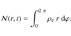
It can be interpreted as an equivalent radial charge density. Indeed

gives the total charge contained in the plasma column at time t. Some examples related to the simulations shown in Fig. 1 are given in Fig. 3. We immediately see that for t<100 (linear stage), the boundary of the plasma column remains unchanged, as discussed before. In a second stage, non-linear effects become important and strongly disturb the boundaries of the plasma annulus. Some very coherent patterns emerge while continuing to rotate. During this period, roughly 100<t<400, the barycenter of the charges moved closer to the inner wall as seen in the left part of Fig. 3. The structure implodes and radial forces shift particles closer to the inner wall. In a final stage, only a few particles have moved outwards, while the main fraction drift close to the inner boundary. Therefore we do not observe any significant diffusion radially outwards.

The situation is very similar for the second run, A2. Here also, the linear regime exists until and the observed growth rate is in close agreement with the linear analysis (red straight line in the right part of Fig. 1). The plasma column stays roughly confined between R₁ and R₂, right part of Fig. 3, no strong density rearrangement is perceptible during this linear phase. During the transition from the linear to the non-linear state, the m=7 structure emerges in the density map as shown in the right part of Fig. 2. Vacuum gaps are formed and seven vortices rotate around the cylinder axis until some of them merge, destabilizing the whole system and shrinking down to the inner wall.

These conclusions apply to all of our runs starting with an initial equilibrium as a plasma annulus. Such behavior is expected because of the confinement theorem which states that on average, the radial excursion of particles is limited due to angular momentum conservation of the system (particles + electromagnetic field), see Davidson (1990).

3.2 Electrosphere

Next, we switch to the results obtained for the electrosphere. As in our previous works, the rotation profile is chosen to mimic the rotation curve existing in the 3D electrosphere. We recall that different analytical expressions for the radial dependence of are chosen mainly by varying the gradient in differential shear as follows

is the neutron star spin and r is normalized to the neutron star radius, R_*. The values used are listed in Table 2. In all cases, starts from corotation with the star at r=1, followed by a sharp increase around r=6 for and a less pronounced gradient around r=10 for . Finally, the rotation rate asymptotes at twice the neutron star rotation speed for large radii, see discussion and figures in Pétri (2007b). In this paper, we show results for the rotation profiles and and a perturbation pattern m=3. Note that the plasma entirely fills the cylinder from W₁=1 to W₂=20 without vacuum gaps. The evolution of the electrostatic energy is shown in Fig. 4. In both cases, the observed growth rates during the linear stage are recovered, in agreement with our linear analysis (compare the black dots with the red straight line) for t<8 in the first run and t<12 in the second case. After this first stage, a transition to a non-linear regime appears. The density perturbation becomes significant and is clearly recognizable in the density map, Fig. 5. Because of small irregularities, the 3 vortices have different rotational speeds, some of them overtake the slowest one and coalesce to a larger single vortex. Eventually, the last vortex is overtaken and in the final situation, only one vortex survives and is dragged towards the neutron star surface (the inner wall). Indeed, inspecting Fig. 6, the highest charge densities are found close to R₁. Here again, we found no significant charge escaping the system to reach the outer wall.

Table 2:   Parameters for the three rotation profiles used to mimic the azimuthal velocity of the plasma in the electrospheric disk.

To summarize these simulations, we demonstrated that our 2D PIC code is able to accurately reproduce the growth rates of the diocotron instability in the linear stage of its development, in accordance with our previous analytical study.

The long period of time in the non-linear stage showed no significant particle diffusion across magnetic field lines. Current flow in the system is not efficient.

Nevertheless, the pulsar magnetosphere is believed to be subject to copious pair creation feeding the electrosphere with highly relativistic, freshly born electrons and positrons. This external source of charge can drastically change the long term behavior of the diocotron instability. That is why in the next and last paragraph, we add a particle injection mechanism into the plasma column (or electrosphere) in order to represent the pair cascade phenomenon in a simple manner.

Table 3:   Eigenvalues  for the electrospheric model , and for some azimuthal modes m.

4 Results with particle injection

The most interesting case is the one assuming that the non-neutral plasma is not isolated but is an open system from which particles can freely enter or exit. Our main focus is on the electrospheric plasma around a neutron star. Close to its surface, due to the high magnetic field intensity, some quantum electrodynamical processes can convert photons into electron-positron pairs. Therefore, in a crude way, we can think of it as a (time-dependent) source feeding the electrosphere with charged particles. Moreover, these charges are responsible for synchrotron and curvature radiation. All these phenomena can drastically affect the behavior of the diocotron instability.

Our goal in this last section is to study in detail the first effect, namely an external source of charges feeding the plasma with a flux of particles. In the most general picture, the spatial and time behavior can be quite complicated. To simplify it, we will assume that the source is located at an arbitrary fixed radius and that the particle flux is constant in time.

In order to investigate the consequences of particle injection into the system, we run the same configurations as above but add a source of particle injected at a radius chosen to be r=2 W₁. Some simulation results are described in the following subsections.

4.1 Plasma column

First, we consider again the plasma annulus with constant charge density trapped between the two conducting walls. In all these runs, we adopt the same conditions as before except that we remove the initial density perturbation. Indeed, we are no longer interested in the linear growth rate. In this way, the exact pattern of the perturbation is not relevant.

The integrated density is shown in Fig. 7 and should be compared with Fig. 3. Note that the color scales are different in both situations. At the beginning of the runs, the plasma annulus rotates around its axis without any significant perturbation. However, around and for the first and second run respectively, the equilibrium configuration has been destroyed and particles shrink to the inner wall. As the simulations start, the location of the source is easily determined on these maps. Particles are injected at a radius r=2 W₁, depicted in the plots by a thin strip. Typical perturbations of the density within the annulus are shown in Fig. 8. In both cases, it seems that the fastest growing mode corresponds to a pattern m=6. The source of particles corresponds to the inner annulus. In the first simulation, in the left figure, there exists a strong interaction between both rings because they show the same azimuthal pattern, at least at the beginning of the non-linear stage. However, this effect is much less pronounced in the second run, on the right, due to the larger separation between the rings. From a careful comparison between the cases with and without injection, we conclude that the radial extension at the end of the simulation is significantly larger (on average) when a source is present. For instance, for the annulus A1, the integrated density does not extend farther than r=2 W₁ when the source is switched off whereas its extension reaches r=5 W₁ when charges are injected. The diffusion process would have been even more extensive if the time span would have been longer. We will make this statement more clear in the discussion of last two sets of runs. The annulus configuration was just a starting point to relate our numerical results to analytically known solutions for the growth rates.

4.2 Electrosphere

Next, we study the behavior of the electrosphere. We take the same configurations as in the previous section and add the source located at r=2 W₁. However, in order to look for particle diffusion farther away than the outer wall located at r=20 W₁, we used an initial box larger with size W₁=1 and W₂=100. This allows us to investigate the large radial excursion of the particle and is a strong indication that charges effectively diffuse across the magnetic field lines.

We investigate the charge density at the end of the runs. A snapshot is given in Fig. 9 for on the left, and on the right. We recall that in the first place, the electrospheric plasma was only filled between r=W₁ and r=20 W₁. In the above pictures, we clearly see a non negligible charge density up to radii larger than (40-50) W₁ or so. This is unambiguous evidence of the efficiency of the diocotron instability to generate a current across the field lines. This fact is supported by inspecting Fig. 10. The integrated density shows a monotonic and regular expansion. During a first rearrangement state, the plasma shrinks and approaches the neutron star surface. This is the meaning of the thin horizontal strip in green-yellow between r=W₁ and r=20 W₁ for time less than roughly t<20. Thus a gap is forming, but after sufficient particles have been injected into the system, these vacuum regions will be replenished and expand even farther radially outwards.

4.3 Vacuum

It is also possible to start with the extreme situation containing no particle, i.e. vacuum. This is the most relevant case to show the efficiency of particle transport across magnetic field lines.

As in the previous cases, we inject particles at r=2 W₁ and let the system evolve in a self-consistent manner according to the electric drift approximation. In the first run, the two conducting walls are relatively close to each other, with W₁=1 and W₂=20 W₁. In this way, we are able to see what is happening in the region close to the injection radius. Depending on the particle injection flux, the plasma column grows radially outwards more or less quickly. As seen in the density snapshot shown in the left part of Fig. 11, during the simulation, particles tend to fill all the space between the two walls. Charge transport across magnetic field lines seems to be very efficient. This is confirmed by inspecting the left part of Fig. 12 in which we see a monotonic increase in outer edge of the integrated charge density. Starting with r around 2 W₁, the plasma annulus has non negligible density at r=13 W₁ at the end of the run.

Finally, in order to clearly view the long term behavior of this diocotron instability, we performed a run with higher resolution as well as larger distance between the conducting walls, W₁=1 and W₂=100. The most relevant results are given in the right part of Figs. 11 and 12, for the density and the integrated density respectively. Here again, for a sufficiently long time, plasma fills the entire vacuum and spreads out over the whole space. The barycenter of the charges drifts to larger and larger radii. This last run is an unambiguous proof demonstrating the crucial role of this non-neutral plasma instability in the modeling of pulsar magnetosphere. Plasma injection in the electrosphere will unavoidably push particles farther away from the neutron star.

4.4 Discussion

We showed that the non-neutral plasma behaves very differently when isolated compared to the situation in which a source of particles is added. In the former case, charges tend to migrate radially inwards, whereas in the latter case, the total charge of the system is not conserved and they are allowed to move radially outwards. This migration to larger distances is induced by the increasing electric repulsion between particles. In the initial (unstable) equilibrium state, the Lorentz force,  , exactly compensates the centrifugal force. The self-field parameter, defined by  , is such that an equilibrium is permitted. For a constant density plasma column it corresponds to . We introduced the plasma frequency (squared) by , the cyclotron frequency by , the mass of the particle (electron or positron in our case), its charge e and the particle density number .

Due to the evident dichotomy between an isolated system for which migration inwards is observed and a system with injection of particles and a radially outwards expansion of the plasma as consequences, we could imagine a situation in between such that no significant radial motion is induced. However, we do not believe that such a regime is reachable, because a charge density increase will inevitably lead to a growing self-field parameter  to values eventually larger than those expected to find an equilibrium solution (which is unity for the constant density plasma column). Remember that the self-field parameter is by definition proportional to the particle density number for a fixed magnetic field intensity. For a plasma column, it is well known that the limit  corresponds to the Brillouin zone and forbids radial confinement above this limit, (Davidson 1990). For this reason, there will be no particle injection rate at which both effects cancel exactly. The secular evolution is always particle diffusion across magnetic field lines to larger distances.

A qualitative and illustrative picture is as follows. For simplicity we take the example of the plasma column without inner voids, uniform density and a constant uniform axial magnetic field. The rotation profile for this column is therefore constant, in other words, the plasma column is in solid body rotation. Because the plasma is confined, the self-field parameter should be less than unity. If some particles were added to the system, keeping the magnetic field constant, the particle number density  increases, as does the self-field parameter by the same proportion. When the Brillouin limit is reached, confinement is broken and particles diffuse to larger radii. A new equilibrium state could be reached in principle whenever  becomes less than unity due to particle dilution in a greater volume. Because the timescale for charge diffusion is much less than the azimuthal rotation period, we can think about a slow, almost adiabatic motion. The column always readjusts to a new ``quasi''-equilibrium state. Thus, electrostatic repulsion is at the heart of the diffusion process.

Finally, we give an estimate for the time evolution of the outer boundary of the system in the following way. In our simulations, at a fixed injection rate, the radial excursion slows down because particles have more space to ``dilute'' in (area in 2D (or volume in 3D) proportional to ) and therefore decreasing more efficiently their density number as r grows. This is indeed observed in our runs. The outer edge of the plasma filled region  can roughly be fitted as evolving in time as a function of . Indeed, assuming that the number of particles injected per unit time is , they should be contained within the radius . Assuming a uniform density within the column, starting from r=0 at t=0, we get , leading to the expected function

This curve is shown as a black solid parabola line in Figs. 10 and 12. The constant factor in front of the was adjusted individually for each run.

5 Conclusion

We designed a 2D electrostatic PIC code to study the long time non-linear evolution of the diocotron instability in a background electromagnetic field with a particular emphasise on the pulsar magnetosphere, where we believe that non-neutral plasmas made of pairs form an electrosphere, known to be diocotron unstable.

We first checked our PIC code by looking for the linear growth stage of the diocotron unstable modes. We found very good agreement between the analytical predictions from the linear analysis and the growth rates derived from our PIC code.

These high growth rates quickly destroy the laminar flow pattern due to differential rotation. Fluid elements merge to form some macroparticles with high density and leaving large vacuum space between them. Moreover, if the system remains isolated, there is no significant particle transport across magnetic field lines. Nevertheless, we found that when adding some external source of charge, there is a net outflow of charge towards the light cylinder. This is believed to come from pair creation in the innermost part of the electrosphere. Non-neutral plasma instabilities like the one presented here are an efficient way to transport particles from regions close to the neutron star to the region where the wind is launched. The connection between the wind and the close magnetosphere still needs to be explained. We think that our work will be a fruitful alternative to existing models.

In this approach, we neglected the magnetic field perturbation induced by the plasma. This assumption is true only for plasma flowing far away from the light cylinder (and inside it). In order to take into account the magnetic field back reaction caused by the plasma, we need to solve the full set of Maxwell equations. This work will be presented in a forthcoming paper and will extend the results already founded in Pétri (2007a) about relativistic stabilization effects on the diocotron instability.

References

• Bettega, G., Cavaliere, F., Cavenago, M., et al. 2007, Phys. Plasmas, 14, 042104 [NASA ADS] [CrossRef] (In the text)
• Birdsall, C., & Langdon, A. 2005, Plasma physics via computer simulation (IOP Publishing)
• Davidson, R. C. 1990, Physics of non neutral plasmas (Addison-Wesley Publishing Company)
• Hockney, R. W., & Eastwood, J. W. 1988, Computer Simulation Using Particles (Institute of Physics Publishing)
• Krause-Polstorff, J., & Michel, F. C. 1985a, MNRAS, 213, 43P [NASA ADS]
• Krause-Polstorff, J., & Michel, F. C. 1985b, A&A, 144, 72 [NASA ADS]
• Michel, F. C. 2005, in Rev. Mex. Astron. Astrofis. Conf. Ser., 27 (In the text)
• Neu, S. C., & Morales, G. J. 1995, in AIP Conf. Ser., 331, 124
• Neukirch, T. 1993, A&A, 274, 319 [NASA ADS] (In the text)
• Oneil, T. M. 1980, Phys. Fluids, 23, 2216 [NASA ADS] [CrossRef]
• O'Neil, T. M., & Smith, R. A. 1992, Phys. Fluids B, 4, 2720 [NASA ADS] [CrossRef]
• Pasquini, T., & Fajans, J. 2002, in Non-Neutral Plasma Physics IV, ed. F. Anderegg, C. F. Driscoll, & L. Schweikhard, AIP Conf. Proc., 606, 453 (In the text)
• Pétri, J. 2007a, A&A, 469, 843 [NASA ADS] [CrossRef] [EDP Sciences]
• Pétri, J. 2007b, A&A, 464, 135 [NASA ADS] [CrossRef] [EDP Sciences]
• Pétri, J. 2008, A&A, 478, 31 [NASA ADS] [CrossRef] [EDP Sciences]
• Pétri, J., Heyvaerts, J., & Bonazzola, S. 2002a, A&A, 387, 520 [NASA ADS] [CrossRef] [EDP Sciences] (In the text)
• Pétri, J., Heyvaerts, J., & Bonazzola, S. 2002b, A&A, 384, 414 [NASA ADS] [CrossRef] [EDP Sciences] (In the text)
• Pétri, J., Heyvaerts, J., & Bonazzola, S. 2003, A&A, 411, 203 [NASA ADS] [CrossRef] [EDP Sciences] (In the text)
• Press, W., Teukolsky, S., & V. W. F. B. 2002, Numerical Recipes in C++ (Cambridge University Press) (In the text)
• Rylov, I. A. 1989, Ap&SS, 158, 297 [NASA ADS] [CrossRef] (In the text)
• Shibata, S. 1989, Ap&SS, 161, 187 [NASA ADS] [CrossRef] (In the text)
• Smith, I. A., Michel, F. C., & Thacker, P. D. 2001, MNRAS, 322, 209 [NASA ADS] [CrossRef] (In the text)
• Spitkovsky, A., & Arons, J. 2002, in Neutron Stars in Supernova Remnants, ed. P. O. Slane, & B. M. Gaensler, ASP Conf. Ser., 271, 81 (In the text)
• Thielheim, K. O., & Wolfsteller, H. 1994, ApJ, 431, 718 [NASA ADS] [CrossRef] (In the text)
• Yatsuyanagi, Y., Kiwamoto, Y., Ebisuzaki, T., Hatori, T., & Kato, T. 2003, Phys. Plasmas, 10, 3188 [NASA ADS] [CrossRef]
• Zachariades, H. A. 1993, A&A, 268, 705 [NASA ADS] (In the text)

All Tables

Table 1:   Eigenvalues  for the constant density plasma annulus, for different modes m and different aspect ratios, d₁ = R₁ / W₂, and d₂ = R₂ / W₂, obtained from the analytical expression found in Davidson (1990).

Table 2:   Parameters for the three rotation profiles used to mimic the azimuthal velocity of the plasma in the electrospheric disk.

Table 3:   Eigenvalues  for the electrospheric model , and for some azimuthal modes m.

All Figures

---

Copyright ESO 2009