On the theory of light curves of video-meteors

P. Pecina; P. Koten

doi:10.1051/0004-6361/200811503

Home

All issues

Volume 499 / No 1 (May III 2009)

A&A, 499 1 (2009) 313-320

Full HTML

Free Access

Issue		A&A Volume 499, Number 1, May III 2009


Page(s)		313 - 320
Section		Planets and planetary systems
DOI		https://doi.org/10.1051/0004-6361/200811503
Published online		30 March 2009

On the theory of light curves of video-meteors

P. Pecina - P. Koten

Astronomical Institute of the Academy of Sciences of the Czech Republic, 251 65 Ondrejov, Czech Republic

Received 11 December 2008 / Accepted 23 February 2009

Abstract
Aims. The aim of the article is to show how the light curve of video-meteors can be described theoretically.
Methods. The method of numerical integration of the system of differential equations describing the motion and ablation of a meteoroid during its atmospheric motion is employed.
Results. We have shown that the modification of the ablation equation and the more general assumptions on the meteoroid cross-section behaviour can lead to a better description of light curves of faint video-meteors. The applied method indicates that the traditionally-used statistical parameter F could be replaced by another one, Levin's parameter $\mu$ , which has a physical meaning.

Key words: meteors, meteoroids

1 Introduction

Since the start of video observations of faint meteors many observed cases have been collected. Light curves of such meteors show different shapes. The location of the point of maximum brightness differs from case to case, see e.g. Fleming et al. (1993), Campbell et al. (2000), Koten et al. (2004), Beech (2007). Several ways have been proposed to describe the shape of a meteor light curve. One of the most frequently used, the F parameter, was introduced by Fleming et al. (1993). They found that light curves of sporadic meteors are nearly symmetrical with only a few cases of flares. Hawkes et al. (1998) analyzed the light curves of Perseid meteors and found that they also produced curves close to symmetrical. We observed the positions of maximum light of meteors that were located both closer to the beginning of the corresponding curve and also closer to its end. The the parameter F describes the location of the maximum brightness on the meteor luminous trajectory. According to classical theory, single body meteoroids should produce light curves characterized by $F \sim 0.7$ (Murray et al. 1999). Leonid meteors observed in 1998, however, produced light curves skewed slightly to the beginning of their luminous trajectory (Murray et al. 1999). Murray et al. (2000) compared meteors belonging to two different filaments of the Leonid meteor stream and found that their properties differ. They applied the dust-ball model and found that the light curves could be synthesized from the intensities produced by individual dust grains. Such an approach was used by Borovicka et al. (2007) to study the atmospheric deceleration and light curves of six Draconid meteors.

The parameter F is purely descriptive. No physical ideas have been used in its formulation. Our aim here is to show that such an approach can be based on physical ideas connected with the physics of meteor motion when generalizing the equations in question. So, we will show how the various shapes of light curves can be described by the extended theory of meteor light curves based on generalized equations describing the atmospheric motion of a meteoroid together with its ablation. We will demonstrate the capability of our approach on cases of some meteors observed by our video cameras. Our aim here is to show that such an approach is capable of yielding correct results for light curves of various shape. The consequences for the physical parameters of meteoroids producing the observed light curves will be left for a future article.

We will use observational data of video-meteors consisting of distances flown by the meteoroid in the atmosphere as a function of time, together with absolute magnitudes at corresponding time points. The parameters will be acquired by a fit of observed distances and magnitudes (intensities) to computed ones.

The presented data were obtained within standard double-station video observations carried out at the Onrejov Observatory. The method is described e.g. in Koten et al. (2006).

2 Theory

The motion and ablation of a meteoroid during its atmospheric flight is usually described by the drag equation (e.g. Bronshten 1983)

$\begin{displaymath}m ~ \dot{v} = - \Gamma ~S ~ \varrho ~ v^2, \end{displaymath}$

(1)

and the ablation one

$\begin{displaymath}\dot{m} = - \frac{\Lambda}{2 Q} ~ S ~ \varrho ~ v^3. \end{displaymath}$

(2)

The dot above the quantities on the left in Eqs. (1) and (2) represents the time derivative. The quantities entering these equations have the following meaning: v and m are the meteoroid instantaneous velocity and mass, S represents the cross-sectional area of the body, $\Gamma$ stands for the drag coefficient and $\Lambda$ represents the heat transfer coefficient. The latent heat of vaporization or fusion of the meteoroid material is designated as Q. The atmospheric density is represented by $\varrho$ . Usually the ablation parameter, $\sigma = \Lambda / (2 Q \Gamma)$ , is also frequently used, so that instead of (2) we have

$\begin{displaymath}\dot{m} = - \sigma ~ \Gamma ~ S ~ \varrho ~ v^3. \end{displaymath}$

(3)

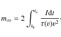
To be able to describe the light effects of meteors we must add the luminosity equation (e.g. Bronshten 1983)

$\begin{displaymath}I = - \frac{\tau}{2} ~ v^2 ~ \dot{m}, \end{displaymath}$

(4)

in which I is the intensity of light produced by the meteor at the time instant, t. The quantity $\tau$ represents the light production efficiency. It is usually considered to be a function of meteoroid velocity. We will employ the velocity dependence put forward by Ceplecha (1988).

Here, we discuss the form of luminosity Eq. (4). Even though Pecina & Ceplecha (1983) proposed that it could be composed of two terms, the former of which is proportional to $v^2 \dot{ m} / 2$ and the latter one to $m v \dot{v}$ , they also showed that it could be given the form of (4) with other definition of the luminous efficiency $\tau$ . The equation with $v^2 \dot{ m} / 2$ expresses the fact that the meteor light is almost entirely produced by species evaporated from the surface of the meteoroid due to its atmospheric ablation. It is, therefore, questionable whether we would observe any meteor event in the case of zero meteoroid ablation. Thus, is the loss of meteoroid kinetic energy due to its deceleration capable of producing a meteor event? We think this is not the case for the faint meteors we are dealing with. Furthermore, micrometeoroids decelerate so much that they are not able to reach the temperature needed for ablation to start and do not produce any light (see, e.g. Bronshten 1983). Therefore, we decided to use the luminosity equation in the form of (4). This was also the point of view of Borovicka et al. (2007) when dealing with the deceleration of Draconid meteors.

When integrating Eq. (4) from the time instant at which a meteor appears, $t_{\rm b}$ , to the one a meteor disappears, $t_{\rm e}$ , we obtain

$\begin{displaymath}m_{\infty} = m_{\rm e} + 2 \int_{t_{\rm b}}^{t_{\rm e}} \frac{I {\rm d} t}{\tau(v) v^2}\cdot \end{displaymath}$

Assuming that the meteoroid is completely destroyed at $t_{\rm e}$ (see, e.g. Bronshten 1983) implying $m_{\rm e} \simeq 0$ we get the relation enabling the evaluation of the initial meteoroid mass

$\begin{displaymath}m_{\infty} = 2 \int_{t_{\rm b}}^{t_{\rm e}} \frac{I {\rm d} t}{\tau(v) v^2}\cdot \end{displaymath}$

(5)

It has the advantage that $m_{\infty}$ obtained in this way does not depend on the theory of the light curve adopted.

To be able to use the above equations to solve practical problems, we must adopt some ideas on the behaviour of S and $\Gamma$ as well as $\sigma$ during the flight of a meteoroid. It is frequently assumed that the shape of a meteoroid does not change during ablation, i.e. the ablation is supposed to be self-similar. Then (e.g. Ceplecha et al. 1998) $S = A ~ m^{2/3} ~ \delta^{-2/3}$ with A being the shape factor and $\delta$ the bulk density of meteoroid material. Introducing the shape-density coefficient, $K = \Gamma ~ A ~ \delta^{-2/3}$ , the system of basic equations now reads

$\begin{displaymath}\dot{v} = - K ~ m^{-1/3} ~ \varrho ~ v^2, \end{displaymath}$

(6)

$\begin{displaymath}\dot{m} = - \sigma ~ K ~ m^{2/3} ~ \varrho ~ v^3. \end{displaymath}$

(7)

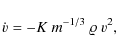
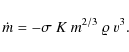
Such equations were recently used also by Borovicka et al. (2007). Both the coefficients K and $\sigma$ were assumed to be constant.

It is known (e.g. Bronshten 1983) that each meteoroid must go through a preablation heating phase before it starts to ablate and, consequently, to produce light. This is not, however, reflected in Eq. (3). Therefore, Pecinová (2005) proposed to modify the ablation equation to read

$\begin{displaymath}\dot{m} = 0 \;~ {\rm for} \; h > h_B, \hspace{2mm} \dot{m} = ... ...~ S ~ (\varrho - \varrho_B) ~ v^3 \;~{\rm for} \; h \leq h_B. \end{displaymath}$

(8)

Here $\varrho_B = \varrho(h_B)$ with h_B representing the height at which the ablation starts. As already stated in the introduction, the assumption of self-similar ablation leads to $F \sim 0.7$ . Since this is generally not the case in observed video meteors we must modify the basic equations to allow for such behaviour of faint meteors. When dealing with the theory of radar meteor range distribution Pecinová & Pecina (2007) entered a similar problem. To overcame it they proposed to adopt Levin's (1956) proposition $S \sim m^{\mu}$ which is more general than the dependence $S \sim m^{2/3}$ . They were successful in obtaining a correct description of range the distributions they observed. Thus, we will make the assumption that

$\begin{displaymath}S = S_{\infty} ~ (m / m_{\infty})^{\mu}, \hspace{5mm} S_{\infty} = A ~ m_{\infty}^{2/3} ~ \delta^{-2/3}, \end{displaymath}$

(9)

where the quantities labelled by $\infty$ refer to their pre-atmospheric values. Whether we are successful will be seen in the next sections. Inserting (9) into (1) and keeping the definition of K leads to

$\begin{displaymath}\dot{v} = - K m_{\infty}^{-1/3} ~ (m / m_{\infty})^{\mu - 1} ~ \varrho ~ v^2. \end{displaymath}$

(10)

The same operation converts (3) into

$\begin{displaymath}\frac{\rm d}{{\rm d} t} \left(\frac{m}{m_{\infty}}\right) = -... ...-1/3} ~ (m / m_{\infty})^{\mu} ~ (\varrho - \varrho_B) ~ v^3. \end{displaymath}$

(11)

On substituting (11) into (4) we get

$\begin{displaymath}I = \frac{1}{2} ~ \sigma ~ K ~ m_{\infty}^{2/3} ~ (\varrho - \varrho_B) ~ \tau( v ) ~ v^5 ~ (m / m_{\infty})^{\mu}. \end{displaymath}$

(12)

The set of Eqs. (10)-(12) is the basis of all our further computations, the results of which we will present in this paper later.

2.1 No deceleration

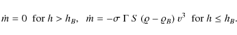
These are the most general equations we will adopt. However, since we deal with faint video meteors whose visible light curves and distances flown usually spread over short regions of heights, their deceleration can be neglected. We can, therefore, integrate Eq. (11) under the assumption $v = v_{\infty}$ . Realizing that

$\begin{displaymath}\frac{{\rm d} h}{{\rm d} t} = -v( t ) ~ \cos z_{\rm R} \end{displaymath}$

(13)

holds generally true, where h is the height at which a meteoroid occur at a time instant, t, and $z_{\rm R}$ is the zenith distance of the meteor radiant, we obtain from (11)

$\begin{displaymath}m = m_{\infty} \left\{1 - (1 - \mu) ~ \frac{K m_{\infty}^{-1/... ...} ~\sigma v_{\infty}^2 ~ F(h, h_B) \right\}^{\frac{1}{1-\mu}}, \end{displaymath}$

(14)

where

$\begin{displaymath}F(h, h_B) = \int_{h}^{h_B} [\varrho(x) - \varrho(h_B)] ~ {\rm d} x. \end{displaymath}$

(15)

This function can easily be constructed from CIRA (1972) in the form of table inside which we can interpolate to reach the value of $\varrho(h)$ that we want. The theoretical light curve follows from the insertion of (14) into (4). We arrive at

$\begin{displaymath}I = c_1 ~ [\varrho(h)-\varrho(h_B)] ~ \left\{1 - (1 - \mu) ~ c_2 ~ F(h, h_B) \right\}^{\mu/(\mu-1)}, \end{displaymath}$

(16)

where now

$\begin{displaymath}c_1 = \sigma K m_{\infty}^{2/3} \tau(v_{\infty}) v_{\infty}^5... ... c_2 = \sigma K m_{\infty}^{-1/3} v_{\infty}^2/ \cos z_{\rm R}.\end{displaymath}$

The parameters c₁, c₂, $\mu$ and h_B are accessible from the solution of the least squares constraint

$\begin{displaymath}\sum_{i=1}^{n} (I^{\rm obs}_{i} - I^{\rm com}_{i})^2 = \min, \end{displaymath}$

(17)

where $I^{\rm com}_{i}$ stands for intensities computed according to (16) and n designates the number of points of the light curve available for our procedure. The method used was described by Pecinová & Pecina (2007). The velocity $v_{\infty }$ can be reached from

$\begin{displaymath}\sum_{j=1}^{n} (l^{\rm obs}_{j} - l_j)^2 = \min, \end{displaymath}$

(18)

where now $l_j = l_r + v_{\infty} t_j$ . The above expressions for c₁ and c₂ imply also that

$\begin{displaymath}\sigma K = \sqrt[3]{2 c_1 c_2^2 \cos^2 z_{\rm R} / \tau(v_{\infty})} / v_{\infty}^3 \end{displaymath}$

and

$\begin{displaymath}m_{\infty} = 2 c_1 /(c_2 \tau(v_{\infty}) v_{\infty}^3 \cos z_{\rm R}). \end{displaymath}$

The last expression also allows the $m_{\infty}$ to be evaluated from (16). This can be compared with the same quantity obtained from (5). Thus, we have two independent ways to obtain $m_{\infty}$ even though we must have in mind that (5) yields this quantity independent of the form of the light curve adopted.

2.2 Deceleration

Even though it holds true that most video meteors do not show noticeable deceleration there have been meteors observed which do slow down. Usually the set of drag and ablation equations is integrated using the first integral obtained when dividing the ablation equation by the drag one. This integral is inserted into the drag equation and further integration yields the dependence of the instantaneous meteoroid velocity, v, on height (see, e.g. Pecina & Ceplecha 1983). However, our corresponding system of Eqs. (10) and (11) does not possess a first integral since dividing (11) by (10) does not cancel out the atmospheric density, $\varrho$ . Therefore, we must solve the set using a numerical integration procedure. We will use the familiar Runge-Kutta integrator of 4th order. Defining the quantity $z = (m / m_{\infty})^{1-\mu}$ , the set of equations to be integrated now reads

$\begin{displaymath}\frac{{\rm d} l}{{\rm d} t} = v, \end{displaymath}$

(19)

$\begin{displaymath}\frac{{\rm d} v}{{\rm d} t} = - K m_{\infty}^{-1/3} ~ \varrho(h) ~ \frac{v^2}{z}, \end{displaymath}$

(20)

$\begin{displaymath}\frac{{\rm d} z}{{\rm d} t} = - \sigma ~ (1- \mu) ~ K m_{\infty}^{-1/3} ~ [ \varrho(h) - \varrho(h_B) ] ~ v^3. \end{displaymath}$

(21)

We must also add

$\begin{displaymath}h = h_{\rm o} - (l - l_{\rm o}) \cos z_{\rm R}, \end{displaymath}$

(22)

providing the relation of heights to distances flown along the meteoroid path. This follows from the geometry of the problem. To be able to integrate (19)-(21) we have to add the proper initial conditions. We will choose the first observed point of the light curve as the one corresponding to time $t_{\rm o}$ . Then $l_{\rm o} = l(t_{\rm o})$ , $v_{\rm o} = v(t_{\rm o})$ and z = 1 for $t = t_{\rm o}$ even though, strictly speaking z = 1 for t corresponding to passing the height h_B. We will neglect this small difference. Again the parameters $l_{\rm o}$ , $v_{\rm o}$ , $K m_{\infty}^{-1/3}$ and $\sigma (1- \mu)$ were computed from (18) using the same procedure as Pecina (2001). Inserting the z-quantity into (12) we get

$\begin{displaymath}I = \frac{1}{2} \tau(v) K m_{\infty}^{-1/3} ~ \sigma ~ m_{\in... ... ~ [\varrho(h) - \varrho(h_B)] ~ v^5 ~ z^{\frac{\mu}{1-\mu}}. \end{displaymath}$

(23)

This can further be used in (17) to get the values of $\sigma$ , h_B and $\mu$ with known $K m_{\infty}^{-1/3}$ by solving (19)-(21) and $m_{\infty}$ from (5). The last three parameters can again be inserted into (19)-(21) to obtain improved values of $l_{\rm o}$ , $v_{\rm o}$ , $K m_{\infty}^{-1/3}$ and $\sigma (1- \mu)$ . The whole iteration can be repeated until the change of the particular parameter drops below the selected level.

We have proceeded so far by solving our problem in two substeps, i.e. minimizing (17) and (18) independently. However, it is useful to combine independent processes into one in the following way. Since l and I have different physical dimensions we must compare their normalized (i.e. dimensionless) quantities. Therefore, we define the following dimensionless quantities

$\begin{displaymath}l_i = l_{\rm o} ~ x(t_i), \;\;\; v_i = v_{\rm o} ~ y(t_i), \;\;\; m_i = m_{\infty} ~ z(t_i)^{1/(1-\mu)}. \end{displaymath}$

(24)

The quantity $l_{\rm o}$ which normalizes the lengths was chosen as the first one measured and was, therefore, fixed. If the reduction programme yielded its zero value then to all lengths we added the difference between the second length and the first one to ensure that $l_{\rm o}$ is nonzero. The set of Eqs. (19)-(21) then converts into

$\begin{displaymath}\frac{{\rm d} x_i}{{\rm d} t} = \frac{v_{\rm o}}{l_{\rm o}} ~ y_i, \end{displaymath}$

(25)

$\begin{displaymath}\frac{{\rm d} y_i}{{\rm d} t} = - K m_{\infty}^{-1/3} ~ v_0 ~ \varrho(h_i) ~ \frac{y_i^2}{z_i}, \end{displaymath}$

(26)

$\begin{displaymath}\frac{{\rm d} z_i}{{\rm d} t} = - \sigma (1- \mu) ~ K m_{\inf... ...{-1/3} ~ v_{\rm o}^3 ~ [\varrho(h_i) - \varrho(h_B)] ~ y_i^3. \end{displaymath}$

(27)

We again add the relation connecting the heights to lengths. This is now

$\begin{displaymath}h_i = h_{\rm o} - l_{\rm o} \cos z_{\rm R} [x(t_i) - 1], \end{displaymath}$

(28)

where $h_{\rm o}$ (fixed) corresponds to $l_{\rm o}$ . From the definition of dimensionless quantities x_i, y_i and z_i it is evident that $x(t_{\rm o})=y(t_{\rm o})=z(t_{\rm o})=1$ . The second part, i.e. the normalized light curve can easily be obtained from (23) to read:

$\begin{displaymath}i_j = i(t_j) = \frac{\tau(v_j)}{\tau(v_{\rm o})} ~ \frac{\va... ...(h_{\rm o})-\varrho(h_B)} \; y_j^5 ~ z_j^{\frac{\mu}{1-\mu}}. \end{displaymath}$

(29)

The least squares condition we now use is

$\begin{displaymath}\sum_{k=1}^{2 n} w_k ~ (q_k^{\rm obs} - q_k^{\rm com})^2 = \min, \end{displaymath}$

(30)

where $q^{\rm obs}_k = x_k^{\rm obs}$ for $1 \leq k \leq n$ and $q^{\rm obs}_k = i_k^{\rm obs}$ for $n+1 \leq k \leq 2 n$ . The quantities with superscript com correspond to x_i from (25)-(27) and i_j from (29). Contrary to (17) or (18) we had to add weights into (30).

$\begin{figure} \par {\includegraphics[width=9cm,clip]{1503fig1.eps} } \end{figure}$

Figure 1:

The distance of the meteoroid from chosen point of its atmospheric trajectory, l, as a function of time, t, for the Quadrantid meteor 2103132. Measured distances are marked by the full squares, the particular variances $l_{\rm obs} - l_{\rm com}$ , outlined along the secondary y-axis, are marked by the asterisks. The linear dependence $l = l_{\rm o} + v_{\infty } t$ , depicted by a full line, was assumed.

Open with DEXTER

The reason for doing this is that the lengths, l_i, and the intensities, I_j, are generally of different accuracy yielding a sum of squares differing by many orders of magnitudes. The measurement of l_i usually gives more precise quantities than the one of magnitudes from which the intensities are derived. Thus, the weights w_k were chosen so that each member of (30) was of the same order as the others. From the constraint (30) the following quantities were evaluated: $v_{\rm o}$ , $K m_{\infty}^{-1/3}$ , $\sigma$ , $\mu$ and h_B together with their standard deviations.

We have hereby completed the theory needed for the description of observed meteors. The next section will deal with the meteors we observed.

3 Application to observed meteors

To apply this theory to observed meteors we proceeded as follows. First, the velocity $v_{\infty }$ was evaluated using (18). Then the parameters c₁ and c₂ assuming $\mu = 2/3$ and $\varrho (h_B)=0$ were evaluated. This corresponds to previously used physical theory. The next step allowed $\varrho (h_B)$ to be nonzero and to be determined as another free parameter. The last step of this procedure allowed $\mu$ to vary and be derived from (17). It is clear that this corresponds to an assumption of zero deceleration. The results we obtained are two cases of Quadrantid video meteors, recorded on January 1, 2002. Figures 1-4 clearly show that when both $\varrho (h_B)$ (i.e. h_B) and $\mu$ are allowed to vary the light curves display the best accordance of theory with observations. The inclusion of $\varrho (h_B)$ improves the course of the light curve at its beginning while the addition of variable $\mu$ does the same inside the whole region of variability of light, namely at the end of the regions. The values of the least squares fit are shown in Table 1. It is worth mentioning that both meteors did not display any noticeable deceleration even though the second one starts to show systematic differences at its end. However, these are so faint that the relevant computational procedure did not give any result here. Also the values of $\mu$ significantly for both cases differ much from the values usually adopted in physical theory of meteors (i.e. $\mu = 2/3$ ).

$\begin{figure} \par {\includegraphics[width=9cm,clip]{1503fig2.eps} } \end{figure}$	Figure 2: The light curves of the meteor from Fig. 1. The curve 1 corresponds to $\mu = 2/3$ and $\varrho (h_B)=0$ , the curve 2 to $\mu = 2/3$ and nonzero $\varrho (h_B)$ , and curve 3 to nonzero $\varrho (h_B)$ and any $\mu$ . For resulting values of these quantities consult Table 1.
Open with DEXTER

$\begin{figure} \par {\includegraphics[width=9cm,clip]{1503fig3.eps} } \end{figure}$	Figure 3: The same as in Fig. 1 but for the Quadrantid meteor 2103169.
Open with DEXTER

$\begin{figure} \par {\includegraphics[width=9cm,clip]{1503fig4.eps} } \end{figure}$	Figure 4: The same as in Fig. 2 but for the Quadrantid meteor 2103169.
Open with DEXTER

Table 1: The mass resulting from the light curve integration, ${m_{\infty }}_{l{\rm c}}$ , the corresponding mass following from the least squares method, ${m_{\infty }}_{l{\rm s}}$ , both in grams, the velocity $v_{\rm o}$ , which is the velocity $v_{\infty }$ in the case of a nondecelerating meteoroid, and the velocity at the beginning of the luminous curve in the case of a decelerating meteoroid, both in km ${{\rm s}}^{-1}$ , $v_{\rm e}$ the velocity at the end of the luminous trajectory, in the same units, K in the CGS system of units, $\sigma$ in $({\rm s} / {\rm km})^2$ , and h_B in km. The abbreviation 0.355e-2 instead of $0.355 \times 10^{-2}$ was used.

$\begin{figure} \par {\includegraphics[width=9cm,clip]{1503fig5.eps} } \end{figure}$	Figure 5: The same as in Fig. 1 but for the meteor 2519197.
Open with DEXTER

$\begin{figure} \par {\includegraphics[width=9cm,clip]{1503fig6.eps} } \end{figure}$	Figure 6: The same as in Fig. 2 but for the meteor 2519197.
Open with DEXTER

$\begin{figure} \par {\includegraphics[width=9cm,clip]{1503fig7.eps} } \end{figure}$

Figure 7:

The distance of the meteoroid from a chosen point of its atmospheric trajectory, l, as a function of time, t, for the meteor 2519197. Measured distances are marked by the full squares, the particular variances $l_{\rm obs} - l_{\rm com}$ , outlined along the secondary y-axis, are marked by the asterisks. The dependence of l on t embodied by Eq. (26) was employed. The resultant function is depicted by the full line.

Open with DEXTER

$\begin{figure} \par {\includegraphics[width=9cm,clip]{1503fig8.eps} } \end{figure}$	Figure 8: The light curve of the meteor from Fig. 7 as a result of application of (30).
Open with DEXTER

$\begin{figure} \par {\includegraphics[width=9cm,clip]{1503fig9.eps} } \end{figure}$	Figure 9: The velocity curve of the meteor from Fig. 7 as a result of application of (30).
Open with DEXTER

$\begin{figure} \par {\includegraphics[width=9cm,clip]{1503figa.eps} } \end{figure}$	Figure 10: The same as in Fig. 5 but for meteor 3729019.
Open with DEXTER

$\begin{figure} \par {\includegraphics[width=9cm,clip]{1503figb.eps} } \end{figure}$	Figure 11: The same as in Fig. 6 but for meteor 3729019.
Open with DEXTER

$\begin{figure} \par {\includegraphics[width=9cm,clip]{1503figc.eps} } \end{figure}$	Figure 12: The same as in Fig. 7 but for meteor 3729019.
Open with DEXTER

$\begin{figure} \par {\includegraphics[width=9cm,clip]{1503figd.eps} } \end{figure}$	Figure 13: The same as in Fig. 8 but for meteor 3729019.
Open with DEXTER

$\begin{figure} \par {\includegraphics[width=9cm,clip]{1503fige.eps} } \end{figure}$	Figure 14: The same as in Fig. 9 but for meteor 3729019.
Open with DEXTER

$\begin{figure} \par {\includegraphics[width=9cm,clip]{1503figf.eps} } \end{figure}$	Figure 15: The same as in Fig. 5 but for meteor 3806030.
Open with DEXTER

$\begin{figure} \par {\includegraphics[width=9cm,clip]{1503figg.eps} } \end{figure}$	Figure 16: The same as in Fig. 6 but for meteor 3806030.
Open with DEXTER

$\begin{figure} \par {\includegraphics[width=9cm,clip]{1503figh.eps} } \end{figure}$	Figure 17: The same as in Fig. 7 but for meteor 3806030.
Open with DEXTER

As already mentioned, some meteors displayed remarkable deceleration. One of these cases is the meteor recorded on May 19, 2002. The computation carried out under the assumption of constant meteor velocity is shown in Figs. 5 and 6. Also from Fig. 6 it is evident that a better description of the observed meteor by the theory is given when both $\varrho (h_B)$ and $\mu$ are parameters of the fit. On the other hand, it is also evident that there is a poorer description at both the beginning and the end of the meteor. Since the time course of variances shows the presence of deceleration, in this case we decided to apply a more thorough model bearing in mind deceleration embodied by (19)-(21) as a first step and (25)-(27) as a second step. The time velocity dependence as well as the light curve are displayed in Figs. 7 and 8. Figure 7 shows no significant systematic time course of variances in accordance with our assumption of velocity variability, as we expected. Moreover, Fig. 8 shows that the inclusion of time variability of the meteoroid velocity into consideration further improves the theoretical light curve which is now much better than in Fig. 6. The correspondence of the theory and observation improved at both ends of the light curve. The graph of velocity we arrive at is presented in Fig. 9. The least squares procedure (30) yielded also the values of the parameters involved in it. They can be found in Table 1. Another meteor displaying deceleration is presented in Figs. 10-14. The velocity curve of 3729019 is depicted in Fig. 14. The case of a decelerating meteoroid with poor data is demonstrated in Figs. 15-19. This is a meteor which was relatively bright and which lasted for much longer than other meteors we have presented. Its complex behaviour is visible both in Fig. 17 where the bump at $t \simeq 1.5$ s can be seen and in Fig. 18 where the confidence of the theoretical light curve with the observed intensities is poorer, namely at the beginning and around the maximum. The velocity curve of 3806030 is depicted in Fig. 19. Table 1 contains all parameters we obtained.

4 Discussion

We have applied the light curve theory to video meteors that are too short to show deceleration, as well as to meteors in which this behaviour displayed very clearly. Both Quadrantid 2103132 and 2103169 as well as 2519197 and 3729019 have short light curves meteors with the light curve maximum of the same order. It is clear that during short time intervals probably no significant changes in l vs. t and light behaviour can manifest. The opposite case 3806030 whose behaviour evidently cannot be described by simple theory. It suffers from many complex changes of its dynamical as well as material properties that are not included in our theory. This meteor may be treated by the theory put forward by Pecina (2001). Our approach may be applied to short and faint video meteors. A first glance at the equations of our theory could lead to the opinion that it is based on a single-body concept. However, the value of $\mu$ different from 2/3 can allow for the situation when the cross-section S is greater than it would be in case of one body. This can, therefore, also allow for fragmentation, for example.

$\begin{figure} \par {\includegraphics[width=9cm,clip]{1503figi.eps} } \end{figure}$	Figure 18: The same as in Fig. 8 but for meteor 3806030.
Open with DEXTER

$\begin{figure} \par {\includegraphics[width=9cm,clip]{1503figj.eps} } \end{figure}$	Figure 19: The same as in Fig. 9 but for meteor 3806030.
Open with DEXTER

Table 1 reveals that the velocity variability can lead to greater values of meteoroid preatmospheric masses when this is not taken into account. The same source of data reveals that the value of $\mu$ can significantly change when the velocity is variable, unlike the opposite case. Also the resultant values of h_B increase when considering variable velocity. The values of the ablation parameter $\sigma$ we have arrived at are quite plausible and can be compared to the corresponding values of bright bolides. However, a closer look at the problem of mutual comparison is not possible here. This we will leave to subsequent work.

5 Conclusions

We have shown that considering nonzero values of $\varrho (h_B)$ and $\mu$ that are to be included in the free parameters to be computed during the least squares fit improves the theoretical description of the observed light curves of video meteors. Further improvement can be made for meteors that clearly decelerate by taking into account of the velocity variability. Our results also indicate that the parameter F introduced by Fleming et al. (1993) can be replaced by Levin's parameter $\mu$ . The closer the light curve maximum to the beginning of the light curve the higher the $\mu$ -value and vice versa. We are aware that this finding must be supported by a much higher number of investigated meteors.

Bronshten (1983) stated that there is still no procedure that yields sufficiently precise values of $\mu$ of observed meteors. We think that our method is capable of providing such values. We plan to study the possible relations of $\mu$ to meteors of various streams based on the theory we presented here.

The approach we have developed is also capable of giving sufficiently precise values of physical parameters of decelerating video meteors such as K, $\sigma$ and h_B which can serve as the basis of further studies devoted to structural characteristics of meteoroids producing these observed meteors.

Acknowledgements

The article has been supported by institutional research plan number AV0Z10030501.

References

Beech, M. 2007, MNRAS, 380, 1649 [NASA ADS] [CrossRef] (In the text)
Borovicka, J., Spurný, P., & Koten, P. 2007, A&A, 473, 661 [NASA ADS] [CrossRef] [EDP Sciences] (In the text)
Bronshten, V. A. 1983, Physics of Meteoric Phenomena (Dordrecht: Reidel), 356 (In the text)
Campbell, M. D., Brown, P., LeBlanc, A. G., et al. 2000, Meteorit. Planet. Sci., 35, 1259 [NASA ADS] (In the text)
Ceplecha, Z. 1988, Bull. Astron. Inst. Czechosl., 39, 221 [NASA ADS] (In the text)
Ceplecha, Z., Borovicka, J., Elford, W. G., et al. 1998, Space Sci. Rev., 84, 327 [NASA ADS] [CrossRef] (In the text)
CIRA 1972, COSPAR International Reference Atmosphere 1972 (Berlin: Academie-Verlag) (In the text)
Fleming, B. D. E., Hawkes, R. L., & Jones, J. 1993, in Proc. Meteoroids and their parent bodies Conf., ed. J. Stohl, & I. P. Williams, Bratislava, Slovakia, 261 (In the text)
Hawkes, R. L., Campbell, M., Babcock, D., & Brown, P. 1998, in Leonid Meteoroid Storm and Satellite Threat Conference, 11 (In the text)
Koten, P., Borovicka, J., Spurný, P., Betlem, H., & Evans, S. 2004, A&A, 428, 683 [NASA ADS] [CrossRef] [EDP Sciences] (In the text)
Koten, P., Borovicka, J., Spurný, P., et al. 2006, MNRAS, 366, 1367 [NASA ADS] (In the text)
Levin, B. Yu. 1956, The physical theory of meteors and meteoric matter in the solar system (Moscow: Publishing House of the Academy of Sciences of the USSR), 293 (in Russian) (In the text)
Murray, I. S., Hawkes, R. L., & Jenniskens, P. 1999, Meteor. Planet. Sci., 34, 949 [NASA ADS] (In the text)
Murray, I. S., Beech, M., Tailor, M., Jenniskens, P., & Hawkes, R. L. 2000, Earth, Moon and Planets, 82, 351 (In the text)
Pecina, P. 2001, in Meteoroids 2001, ed. B. Warmbein, SP-495, ESA, Kiruna, Sweden, 271 (In the text)
Pecina, P., & Ceplecha, Z. 1983, Bull. Astron. Inst. Czechosl., 34, 102 [NASA ADS] (In the text)
Pecinová, D. 2005, Ph.D. Theses, Study of physical characteristics of meteor showers based on Ondrejov radar observations, Charles University, Prague (In the text)
Pecinová, D., & Pecina, P. 2007, Contrib. Astron. Obs. Skalnaté Pleso, 37, 83 [NASA ADS] (In the text)

All Tables

Table 1: The mass resulting from the light curve integration, ${m_{\infty }}_{l{\rm c}}$ , the corresponding mass following from the least squares method, ${m_{\infty }}_{l{\rm s}}$ , both in grams, the velocity $v_{\rm o}$ , which is the velocity $v_{\infty }$ in the case of a nondecelerating meteoroid, and the velocity at the beginning of the luminous curve in the case of a decelerating meteoroid, both in km ${{\rm s}}^{-1}$ , $v_{\rm e}$ the velocity at the end of the luminous trajectory, in the same units, K in the CGS system of units, $\sigma$ in $({\rm s} / {\rm km})^2$ , and h_B in km. The abbreviation 0.355e-2 instead of $0.355 \times 10^{-2}$ was used.

All Figures

$\begin{figure} \par {\includegraphics[width=9cm,clip]{1503fig1.eps} } \end{figure}$	Figure 1: The distance of the meteoroid from chosen point of its atmospheric trajectory, l, as a function of time, t, for the Quadrantid meteor 2103132. Measured distances are marked by the full squares, the particular variances $l_{\rm obs} - l_{\rm com}$ , outlined along the secondary y-axis, are marked by the asterisks. The linear dependence $l = l_{\rm o} + v_{\infty } t$ , depicted by a full line, was assumed.
Open with DEXTER
In the text

$\begin{figure} \par {\includegraphics[width=9cm,clip]{1503fig2.eps} } \end{figure}$	Figure 2: The light curves of the meteor from Fig. 1. The curve 1 corresponds to $\mu = 2/3$ and $\varrho (h_B)=0$ , the curve 2 to $\mu = 2/3$ and nonzero $\varrho (h_B)$ , and curve 3 to nonzero $\varrho (h_B)$ and any $\mu$ . For resulting values of these quantities consult Table 1.
Open with DEXTER
In the text

$\begin{figure} \par {\includegraphics[width=9cm,clip]{1503fig3.eps} } \end{figure}$	Figure 3: The same as in Fig. 1 but for the Quadrantid meteor 2103169.
Open with DEXTER
In the text

$\begin{figure} \par {\includegraphics[width=9cm,clip]{1503fig4.eps} } \end{figure}$	Figure 4: The same as in Fig. 2 but for the Quadrantid meteor 2103169.
Open with DEXTER
In the text

$\begin{figure} \par {\includegraphics[width=9cm,clip]{1503fig5.eps} } \end{figure}$	Figure 5: The same as in Fig. 1 but for the meteor 2519197.
Open with DEXTER
In the text

$\begin{figure} \par {\includegraphics[width=9cm,clip]{1503fig6.eps} } \end{figure}$	Figure 6: The same as in Fig. 2 but for the meteor 2519197.
Open with DEXTER
In the text

$\begin{figure} \par {\includegraphics[width=9cm,clip]{1503fig7.eps} } \end{figure}$	Figure 7: The distance of the meteoroid from a chosen point of its atmospheric trajectory, l, as a function of time, t, for the meteor 2519197. Measured distances are marked by the full squares, the particular variances $l_{\rm obs} - l_{\rm com}$ , outlined along the secondary y-axis, are marked by the asterisks. The dependence of l on t embodied by Eq. (26) was employed. The resultant function is depicted by the full line.
Open with DEXTER
In the text

$\begin{figure} \par {\includegraphics[width=9cm,clip]{1503fig8.eps} } \end{figure}$	Figure 8: The light curve of the meteor from Fig. 7 as a result of application of (30).
Open with DEXTER
In the text

$\begin{figure} \par {\includegraphics[width=9cm,clip]{1503fig9.eps} } \end{figure}$	Figure 9: The velocity curve of the meteor from Fig. 7 as a result of application of (30).
Open with DEXTER
In the text

$\begin{figure} \par {\includegraphics[width=9cm,clip]{1503figa.eps} } \end{figure}$	Figure 10: The same as in Fig. 5 but for meteor 3729019.
Open with DEXTER
In the text

$\begin{figure} \par {\includegraphics[width=9cm,clip]{1503figb.eps} } \end{figure}$	Figure 11: The same as in Fig. 6 but for meteor 3729019.
Open with DEXTER
In the text

$\begin{figure} \par {\includegraphics[width=9cm,clip]{1503figc.eps} } \end{figure}$	Figure 12: The same as in Fig. 7 but for meteor 3729019.
Open with DEXTER
In the text

$\begin{figure} \par {\includegraphics[width=9cm,clip]{1503figd.eps} } \end{figure}$	Figure 13: The same as in Fig. 8 but for meteor 3729019.
Open with DEXTER
In the text

$\begin{figure} \par {\includegraphics[width=9cm,clip]{1503fige.eps} } \end{figure}$	Figure 14: The same as in Fig. 9 but for meteor 3729019.
Open with DEXTER
In the text

$\begin{figure} \par {\includegraphics[width=9cm,clip]{1503figf.eps} } \end{figure}$	Figure 15: The same as in Fig. 5 but for meteor 3806030.
Open with DEXTER
In the text

$\begin{figure} \par {\includegraphics[width=9cm,clip]{1503figg.eps} } \end{figure}$	Figure 16: The same as in Fig. 6 but for meteor 3806030.
Open with DEXTER
In the text

$\begin{figure} \par {\includegraphics[width=9cm,clip]{1503figh.eps} } \end{figure}$	Figure 17: The same as in Fig. 7 but for meteor 3806030.
Open with DEXTER
In the text

$\begin{figure} \par {\includegraphics[width=9cm,clip]{1503figi.eps} } \end{figure}$	Figure 18: The same as in Fig. 8 but for meteor 3806030.
Open with DEXTER
In the text

$\begin{figure} \par {\includegraphics[width=9cm,clip]{1503figj.eps} } \end{figure}$	Figure 19: The same as in Fig. 9 but for meteor 3806030.
Open with DEXTER
In the text

Current usage metrics show cumulative count of Article Views (full-text article views including HTML views, PDF and ePub downloads, according to the available data) and Abstracts Views on Vision4Press platform.

Data correspond to usage on the plateform after 2015. The current usage metrics is available 48-96 hours after online publication and is updated daily on week days.

Initial download of the metrics may take a while.