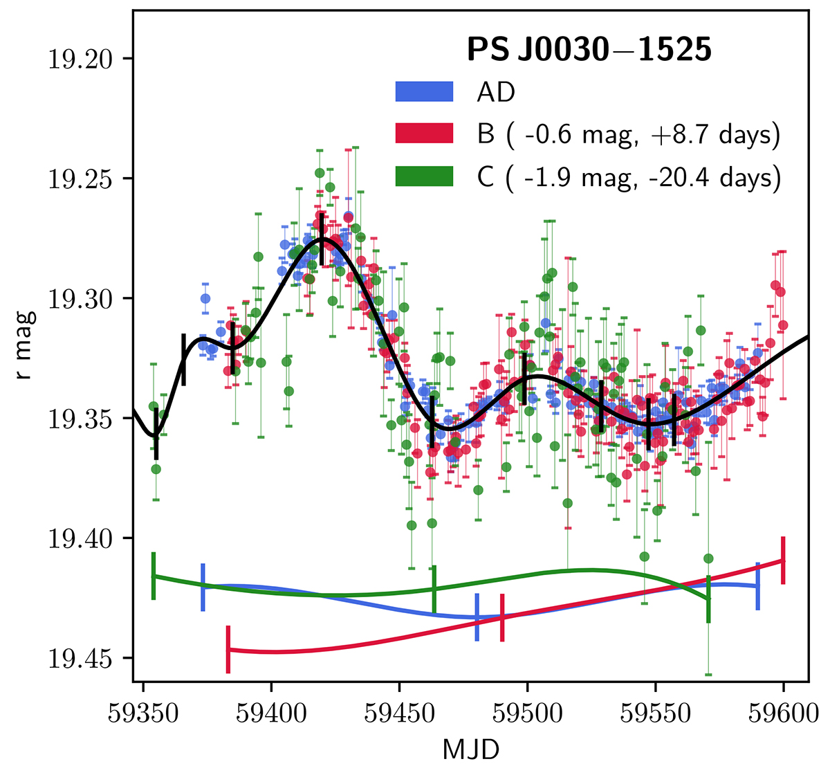
Fig. 7.
Download original image
Curve matching example, in which a single spline (in black) matches all curves simultaneously. Due to microlensing in particular, which adds independent lower-frequency variations to each curve, the curves could not be matched in this way with time and magnitude shifts only. Thus, an extra modulation is applied to each separately. These modulations are represented by lower order splines, displayed at the bottom. Physically, the black spline models the intrinsic variations of the source, while the coloured splines undo the effects of microlensing. Linking with the notation of Sect. 4, Mext is here a cubic spline with a single internal knot of fixed position, and Nint = 9. To determine a time delay and its uncertainty, this matching was repeated thousands of times with artificially further-modulated curves (mimicking microlensing), other realisations of the noise, and different freedoms given to the splines. What this matching is like for the other targets can be found in a Jupyter notebook. This notebook is part of the repository containing the photometry extracted herein and the code to estimate the time delays.
Current usage metrics show cumulative count of Article Views (full-text article views including HTML views, PDF and ePub downloads, according to the available data) and Abstracts Views on Vision4Press platform.
Data correspond to usage on the plateform after 2015. The current usage metrics is available 48-96 hours after online publication and is updated daily on week days.
Initial download of the metrics may take a while.