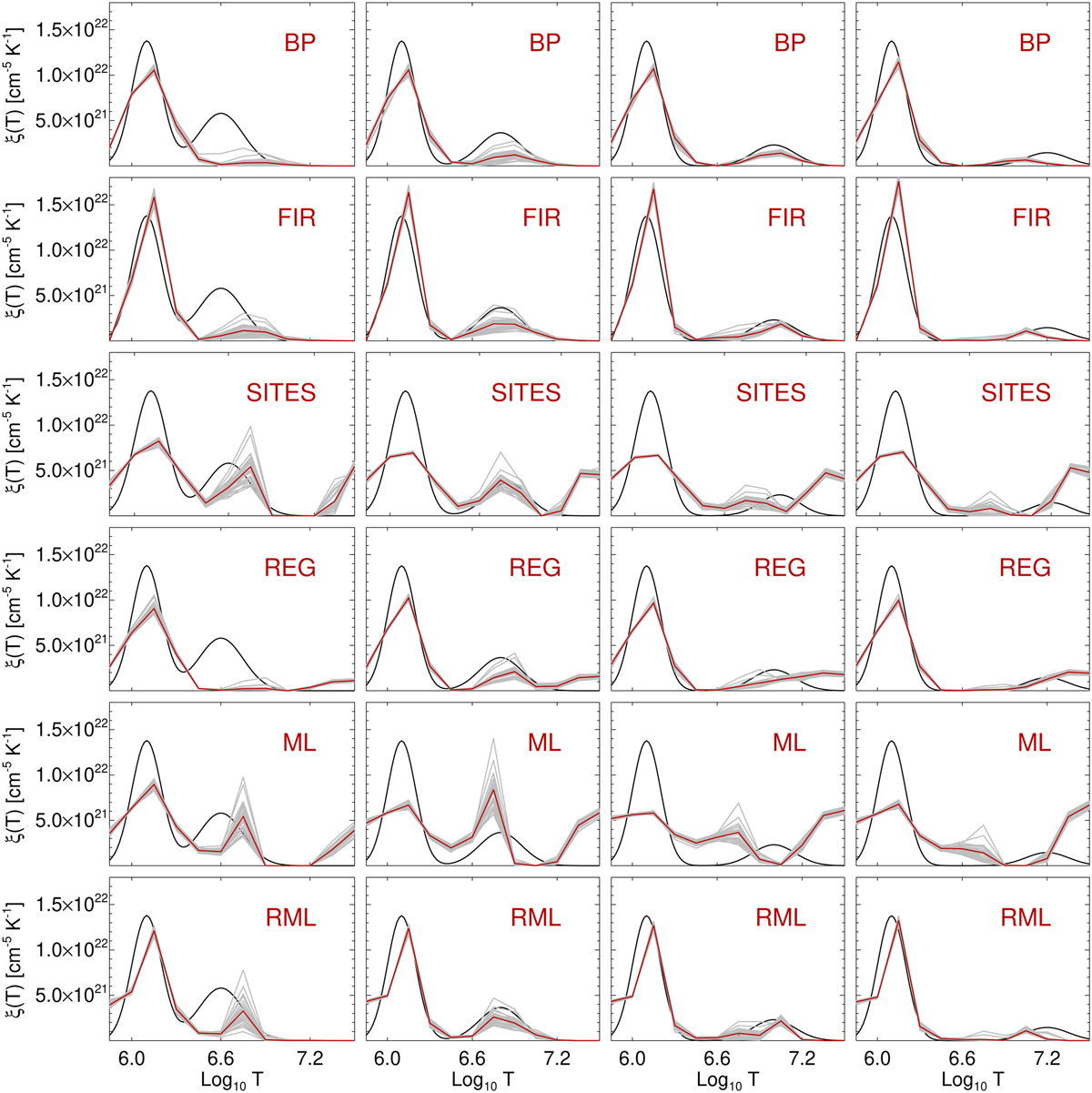
Results of the double-Gaussian simulation tests. From top to bottom: Reconstructions of a simulated double Gaussian ξ(T) profile by means of the basis pursuit (BP) technique (Cheung et al. 2015), the FIR inversion method of Plowman et al. (2013), the iterative SITES technique (Morgan & Pickering 2019), the regularization technique of Hannah & Kontar (2012, REG), the ML method defined in Eq. (18), and finally our proposed RML technique. The black solid lines represent the “ground truth” configurations, which consist of double Gaussian profiles. The left Gaussian has a total Emission Measure EM = ∫ξ(T) dT = 10²⁸ cm⁻⁵ and a standard deviation of 0.1 dex, and is centered on log₁₀ T_c = 6.1, while the right Gaussian has a total Emission Measure EM = ∫ξ(T)dT = 2 × 10²⁸ cm⁻⁵ and a standard deviation of 0.15 dex, and is centered on (from left to right) log₁₀ Tc = 6.6, 6.8, 7.0 and 7.2. The gray lines represent reconstructions from 25 different realizations of Poisson noise affecting the data; the red lines represent the mean values of these 25 reconstructions. The ξ(T) profiles are plotted as a function of the (base 10) logarithm of the temperature (K).