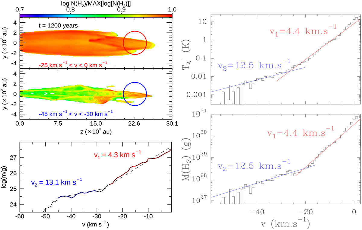
Left: model DR_P at t = 1200 yr under an inclination of 10° (towards theobserver). Top: map of H₂ column density for j_mix = 0.9, in the velocity intervals –[1–25 km s⁻¹] (top) and –[30–45 km s⁻¹] (bottom). The 5000 au aperture used to extract the mass–velocity distribution is drawn by a circle. Bottom: molecular mass–velocity distribution extracted at position A4. We have superposed the best exponential fits m(v) ∝exp(−v∕v_i) to the components associated with velocity intervals –[1–25 km s⁻¹] (red) and –[30–45 km s⁻¹] (blue). The exponent value v_i is given for both velocity intervals. Right: ASAI observations of L1157-B1. Top: intensity–velocity distribution obtained in the CO J = 2–1 towards shock position B1 in an aperture of about 4000 au (11′′ at the distance to the source). The line profile is fitted by a linear combination of two exponential functions g₁ ∝ exp(−v∕12.5) (blue), g₂ ∝ exp(−v∕4.4) (red) (from Lefloch et al. 2012). Bottom: associated mass–velocity distribution, adopting a standard CO-to-H₂ abundance ratio and the excitation conditions derived by Lefloch et al. (2012) for the velocity components g₁ and g₂.