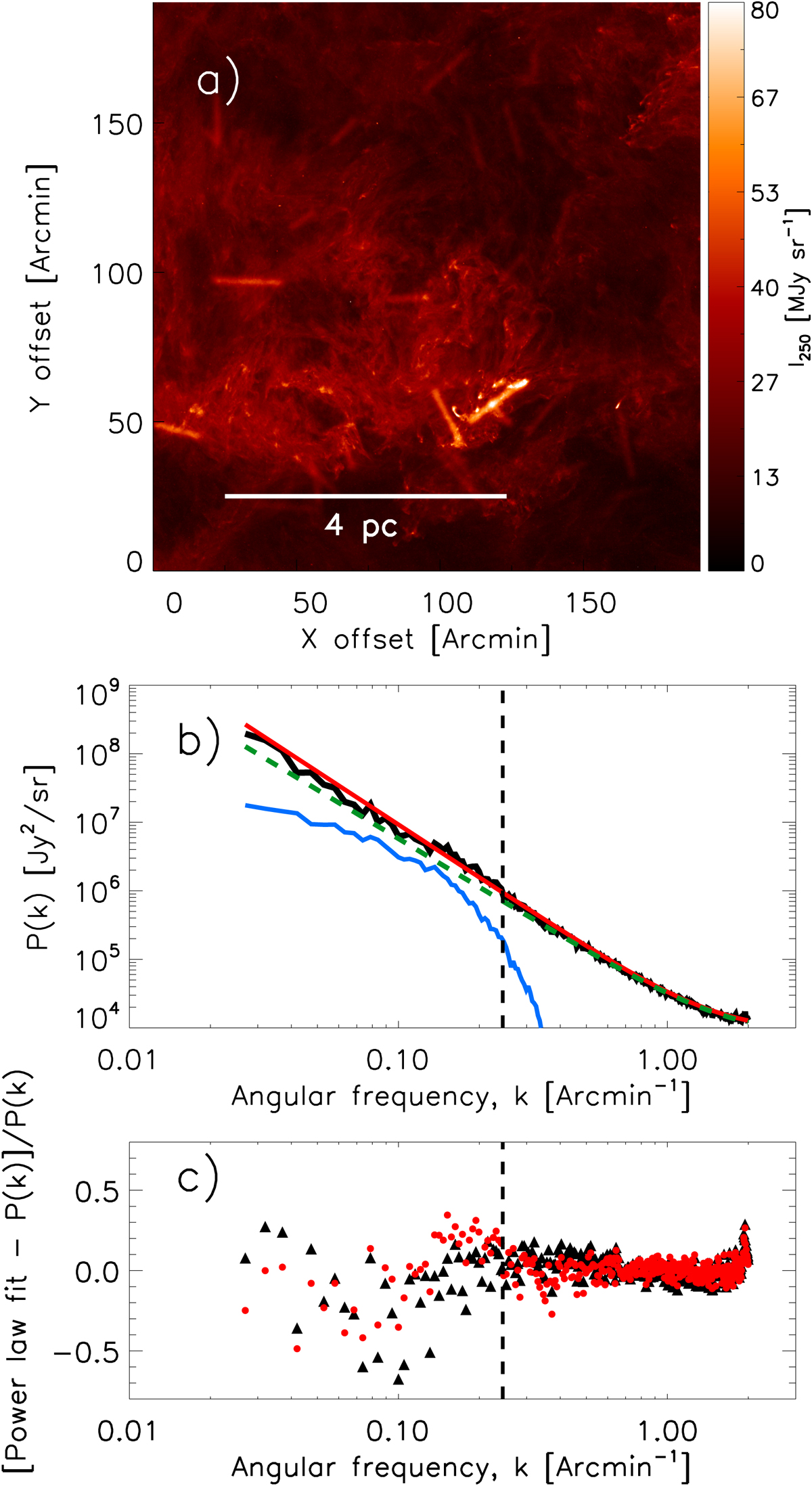
Same as Fig. 4 for synthetic filaments added to a filament-subtracted image of Polaris obtained with getfilaments (Men’shchikov 2013). The population of synthetic filaments is the same as that in Fig. 4. Panel b: green dashed line shows the best power-law fit to the power spectrum of the filament-subtracted background image of Polaris (with no synthetic filaments), which has a slope of γ = −2.4 ± 0.1. The solid black curve shows the total power spectrum of the filament-subtracted image plus synthetic filaments. The best-fit power-law (red curve) has a slope of γ = −2.5 ± 0.1, slightly steeper than the slope of the power spectrum of the filament-subtracted background image (dashed green curve). The blue curve is the power spectrum of the image containing only synthetic filaments. Panel c: black triangles are the same as in Fig. 3c and the red dots show the residuals between the best-fit power-law model and the power spectrum of the image including synthetic filaments. The of the residuals between k_min <  k <  1.5 k_fil is 0.034. The vertical dashed line marks the angular frequency k_fil ∼ (0.6/θ_fil) corresponding to the characteristic ∼0.1 pc width of the synthetic filaments.