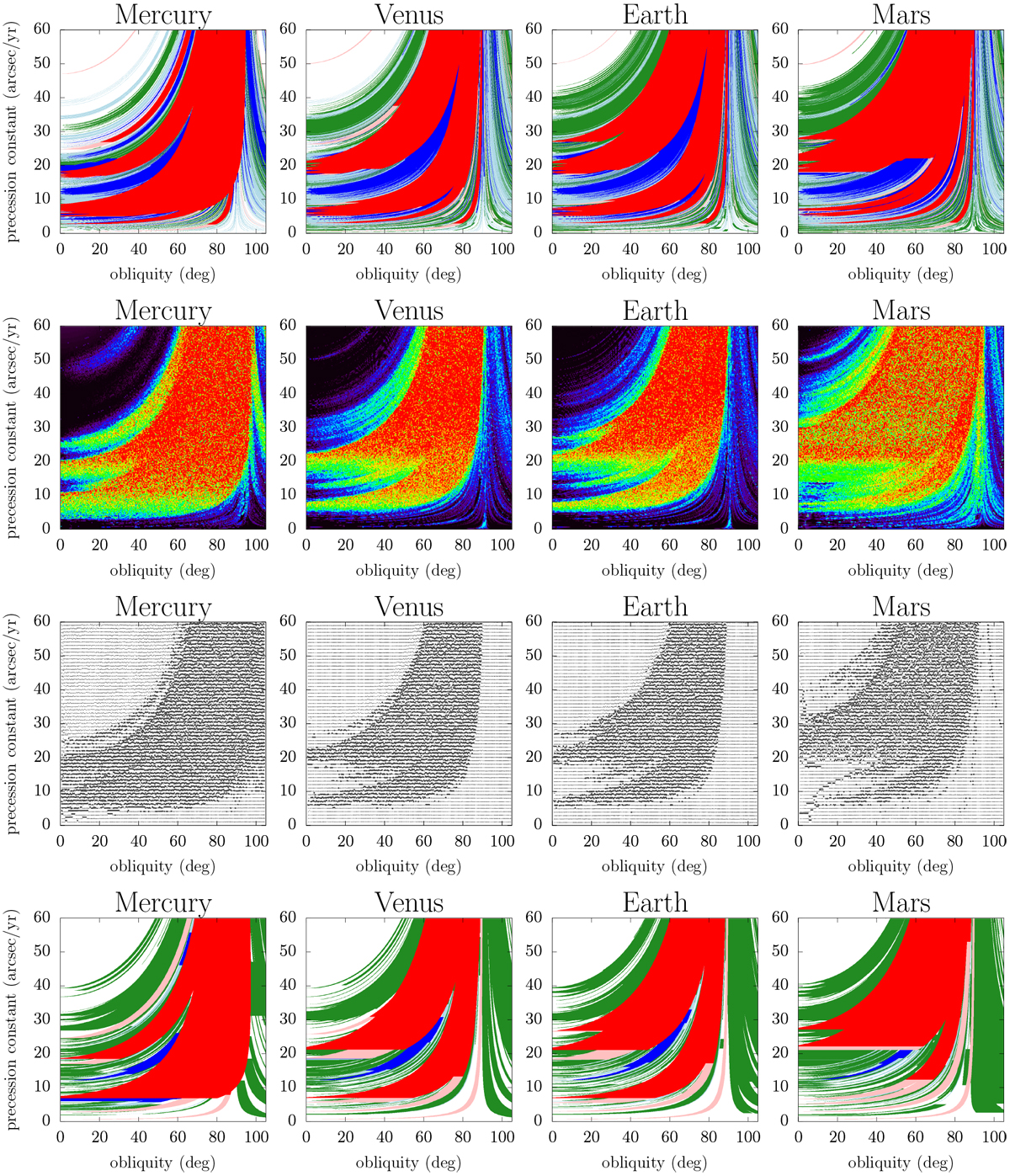
Top row: estimate of the chaotic regions of the spin dynamics as the superposition of secular spin-orbit resonances. The orbitalevolution of each planet is approximated by the synthetic representation of Laskar (1990), as detailed in Appendix F. Light-red and dark-red regions represent the first-order resonances and their overlaps, respectively(Colombo’s top Hamiltonian, Sect. 2.2); light-blue and dark-blue regions represent the second-orderresonances and their overlap (Sect. 2.4); and green regions represent the overlap of third-order resonances. The non-overlapping third-order resonances are not indicated because they are very thin and thus unimportant for a global picture of the dynamics. Second row: as a comparison, the system given by Eq. (1) is integrated numerically with the same orbital model (quasi-periodic decomposition of Laskar 1990), and a frequency map analysis is performed to locate the chaotic zones. The colour scale goes from black (no chaos), to red (strong chaos). Third row: same maps obtained from a more detailed model in which the orbital evolution is directly taken from a numerical integration (adapted from Laskar & Robutel 1993). In the weakly chaotic zones, the dots are shifted vertically according to the level of chaos; in the strongly chaotic zones, they are plotted in boldface. Bottom row: same as top row, but the long-term orbital evolution of each planet is approximated by the Lagrange-Laplace system (Sect. 3.1). The eight planets of the solar system are included, with the initial conditions of Bretagnon (1982).