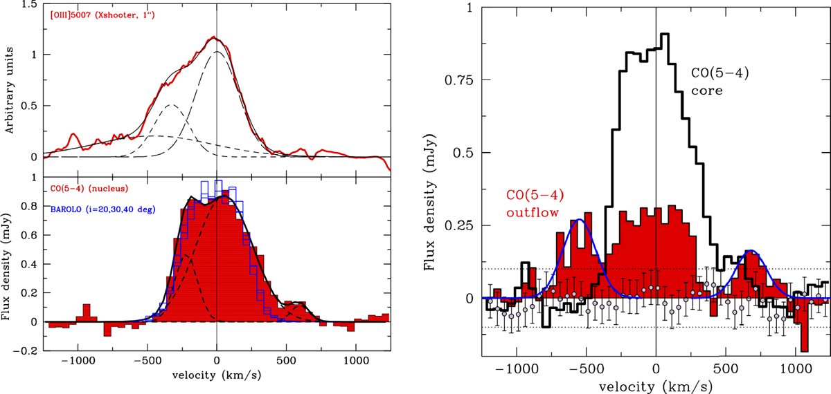
Left panel: [OIII] line profile (red curve taken from Perna et al. (2015); upper) and CO(5 − 4) line profile (red filled histogram; lower), both extracted from the ~ 1″ diameter area shown in Fig. 1. In contrast to Fig. 2, the continuum-subtracted CO(5 − 4) spectrum is binned at 50 km s⁻¹. The blue curves overplotted on the CO(5 − 4) data represent the spectral profile extracted from the model data cube obtained with ^3DBAROLO (see Sect. 4), assuming 20, 30, and 40^° inclination. The dashed lines represent the set of Gaussian components needed to reproduce the line profiles. Right panel: CO(5 − 4) spectrum extracted from a polygonal region encompassing the 1σ contours shown in the left panel of Fig 9 (red histogram extracted from the data cube obtained with a natural weighting scheme). We also show the ±1σ level (dotted lines), the average of three noise spectra taken randomly in the field over a region with the same area and shape as that of the outflow (purple circles), and, for reference, the CO(5 − 4) spectrum taken from the left panel as well (open histogram). The blue curves represent our Gaussian fit to the blue and red excesses at around v ~−600 and v ~ 700 km s⁻¹, respectively. In all panels, the v = 0 position is denoted by a solid vertical line.