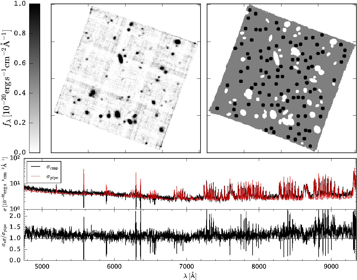
Illustration of the empirical noise calculation procedure. Shown is the case in the MUSE-Wide pointing MUSE-candels-cdfs-06. The top left panel shows a white-light image created by summing over all spectral layers and subsequent division by the spectral range. In the top right panel we show the 100 random 2′′ diameter apertures (black) and the avoided regions (white) because of the presence of continuum bright objects (sources with m_F814< 25 mag in Guo et al. 2013). In the bottom panels we compare the width of the distribution of the flux values extracted in the 100 apertures for each spectral layer σ_emp (black curve) normalised to one spectral pixel to the corresponding aperture average from the pipeline produced variance cube σ_pipe (red curve).