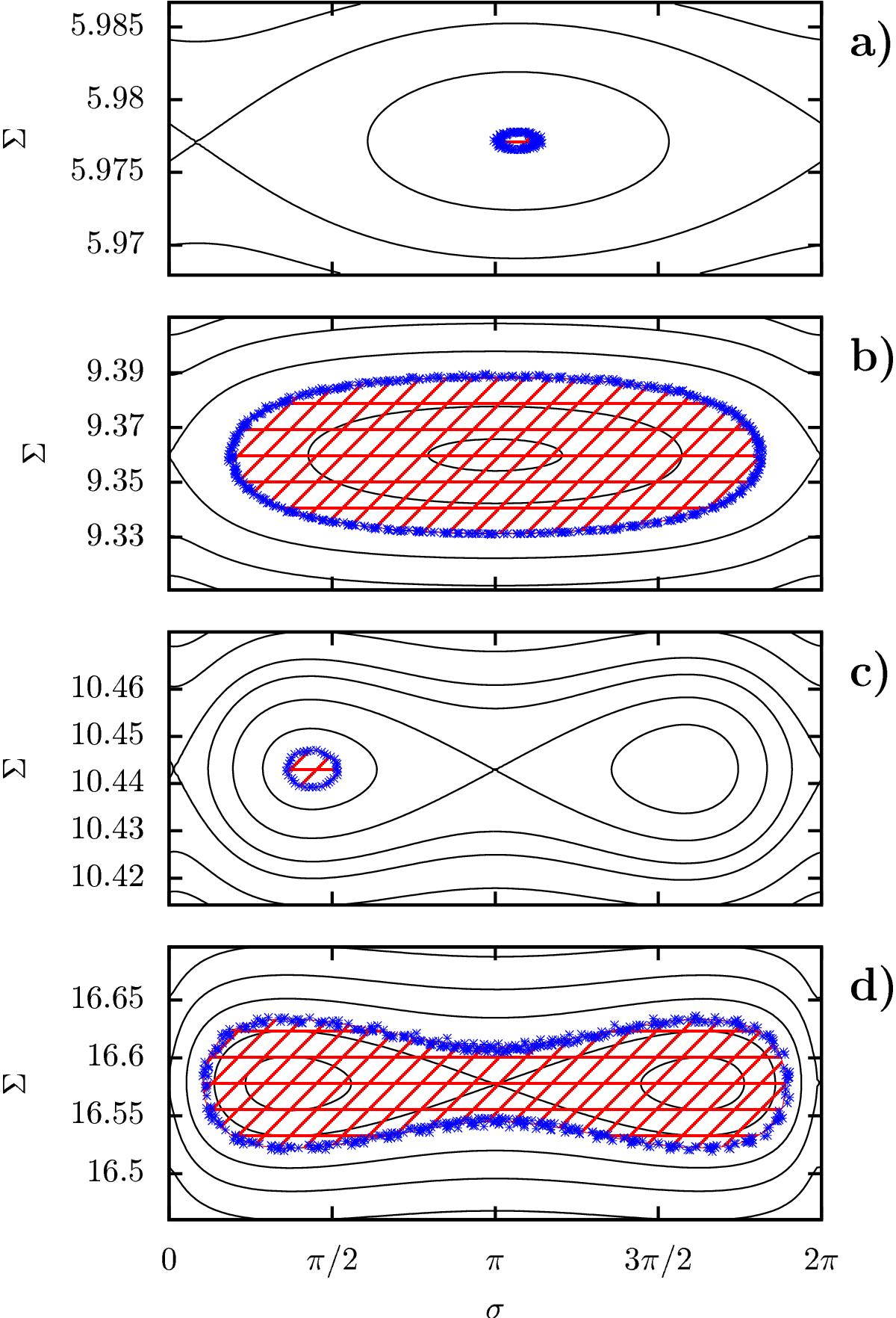
Computation of the secular constant of motion J from the filtered numerical integration. The examples shown are (from top to bottom): 82075, 119068, 2008 ST₂₉₁ and 136120. See Table 1 for the corresponding resonances. The axes are the resonant angle σ from Eq. (1) (rad), and its conjugated momentum Σ from Eq. (3) (au² rad yr^-1). The blue crosses come from the filtered output, whereas the red hatched area is equal to the quantity −2πJ used to construct the secular model. The black lines in the background are the level curves of (2)with (U,u) fixed.Various cases are shown: a), c) small area; b), d) large area; a), b) single resonance island; c), d) double resonance island; a), b) simple oscillations; c) asymmetric oscillations; d) horseshoe oscillations.