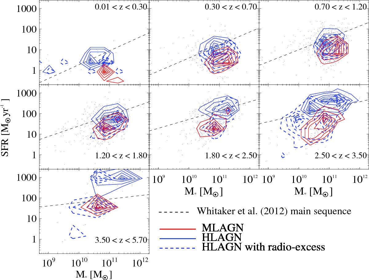
Distribution of HLAGN and MLAGN in the SFR–M_⋆ plane as a function of redshift (black dots). The 2D density contours highlight the distribution of MLAGN (red), HLAGN (blue), and the subsample of HLAGN with radio excess (blue dashed contours), respectively. The 2D density contours enclose the sources (from outer to inner contours) with density levels >35, >50, >68, >80, >90, and >95% of the maximum 2D density. The black dotted lines indicate the MS relation (Whitaker et al. 2012) at different redshifts. The highest redshift bin contains only a few tens of sources, which explains the noise seen in the 2D density contours.