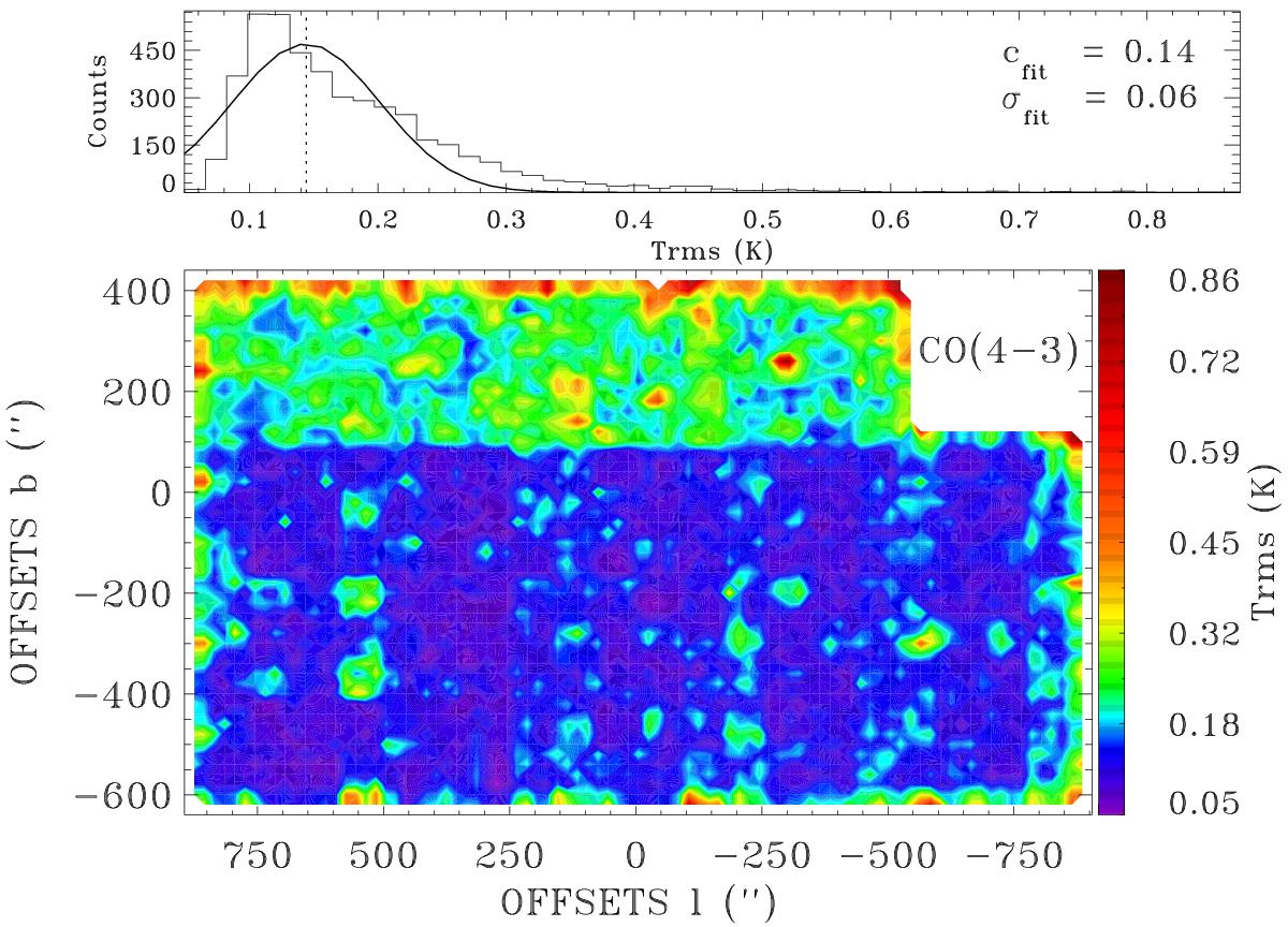
CO(4−3) noise distributions. The spatial noise distribution and the histogram of the noise distribution are shown. The noise distribution spatial map is centred at l = 0°, b = 0°. From the spatial map, the noise is higher at the edges of the map, as expected given the small number of spectra at the borders with which to calculate the resampled spectrum. From the histogram, a Gaussian fit (solid curve) shows the typical noise of the map C_fit (Gauss centre shown as a vertical dashed line) and the standard deviation of the distribution σ_fit.