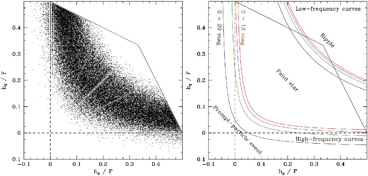
Left panel: example across-scan (AC) rejection plot, based on the along-scan-integrated flux vector h, for 50 000 single stars (Sect. 3.1) with magnitudes between G = 19.5 and 20 mag (so that typical flux values are F ~ 140 LSB). Stars with a symmetric PSF which are centred in an SM sample fall on the diagonal 1:1 relation. Stars with sharp PSFs fall close to the origin whereas stars with broad PSFs move diagonally up towards the vertex h₀/F = h₂/F = 1/3. When, for a given PSF size, the PSF centring inside the sample is varied, objects move on a hyperbolic curve either towards the top left or towards the bottom right. In the absence of Poisson noise, stars with different brightnesses occupy the same hyperbolic curves. The effect of Poisson noise is to broaden this curve into a hyperbolically-shaped cloud; the spread is larger for faint stars since Poisson noise is relatively more important for faint than for bright stars. This effect, combined with background-subtraction errors, can lead to negative h₀ and/or h₂ values and hence negative data points, in particular for faint stars. Because of the finite number of LSB units in the working window (F ~ 140 LSB), discretisation effects in h₀/F and h₂/F can be seen in the data. Right panel: example across-scan rejection plot with high- and low-frequency curves associated with, respectively, Eqs. (5) and (6) for fluxes F associated with magnitudes G = 12 (red), 18 (magenta), 19 (green), and 20 (blue) mag. The saturation and truncation operators from, respectively, Eqs. (3) and (4) have not been included in the curves; they therefore merely serve illustration purposes. The curves, defined through the user-defined VPA parameters (a,b,c,d,e)_{HF, ↑} and (a,b,c,d,e)_{LF, ↑} which have here – for illustration – been set to the functional-baseline values, are flux dependent although the effect of flux on the curves is minimal for bright stars (the curves essentially superimpose for stars brighter than G ~ 15 mag). The upper set of curves is referred to as low frequency (LF) whereas the lower set of curves is referred to as high frequency (HF). Objects above the upper curve are labelled “ripple” while objects below the lower curve are labelled “prompt-particle event”; objects in between the lower and upper curves – for the applicable flux level – are labelled “faint star”. Gaia’s on-board object detection is based on an along-scan rejection plot using shape vector v (not shown) and an across-scan rejection plot using shape vector h (shown here). The domain of possible h₀/F and h₂/F values is limited by the definition of a local maximum in the VPAs: since a local maximum is defined as h₁ ≥ h₀ and h₁>h₂ (Eq. (2)), the maximum values that h₀/F and h₂/F can (asymptotically) take are 1/3 each. Similarly, the maximum value that each of them can (asymptotically) take is 1/2, with the other then (asymptotically) taking the value 0. More generally, Eq. (2) induces boundaries on the rejection plot (solid lines), below which a data point must fall to obey the VPA local-maximum definition.