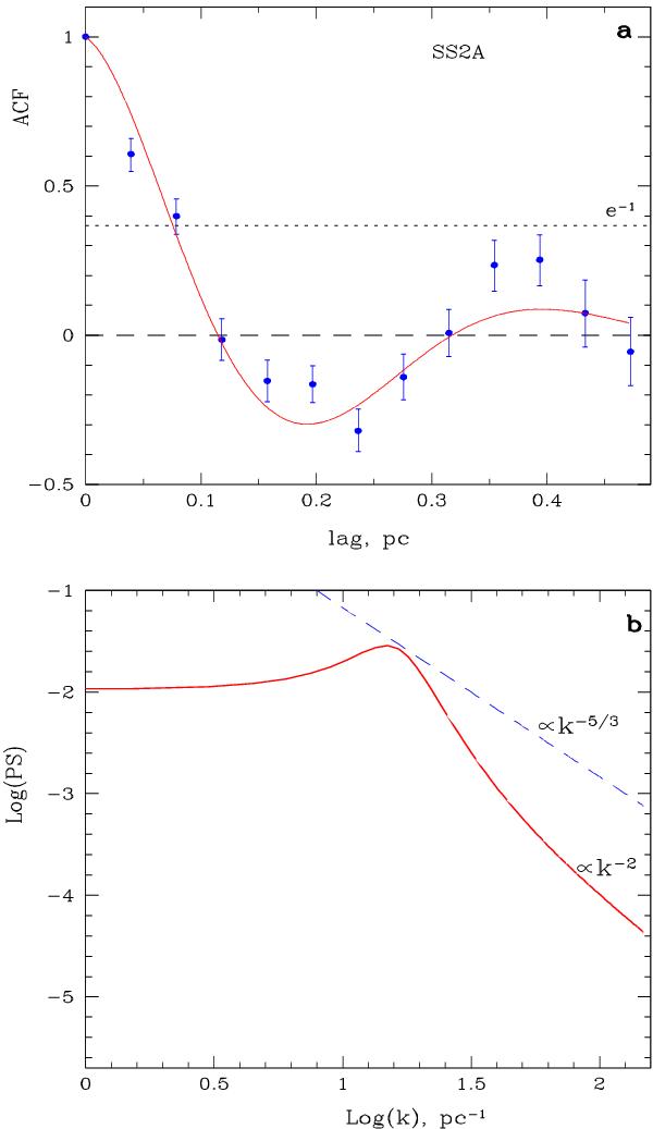
Autocorrelation function (ACF) and corresponding power spectra (PS) of the turbulence in SS2A. a) The solid line indicates the best fit of the azimuthally averaged ACF (filled circles with 1σ error bars) to a model of decaying oscillations as discussed in Sect. 4.3. The zero and e^-1 levels are shown by long- and short-dashed lines. The lag is given in pc for the distance to the source D = 203 pc. b) The power spectrum of velocity P_1D(k) (solid line) assumes homogeneous and isotropic turbulence (the wavenumber ). The spectrum is calculated using Eq. (13). Note the turnover of the PS at a scale of ≈0.06 pc (k_m ≈ 17 pc^-1), where energy is being injected into the system. For comparison, the theoretical PS of a pure Kolmogorov cascade of incompressible turbulence is shown by a dashed line. The Kolmogorov power-law index is κ_1D = −5/3, while the model value is −2 in the inertial range at high wavenumbers, k > k_m.