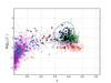
Fig. A.1
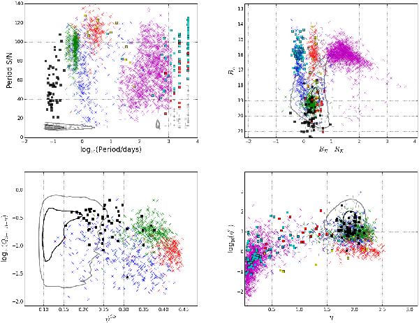
2D scatter plots of variability features of the training set explained in Sect. 3.1. DSCTs: black squares, RRLs: green x, CEPHs: red x, EBs: blue x, T2CEPHs: yellow squares, LPVs: magenta x, QSOs: red squares, BVs: cyan squares, and NonVars: grey crosses. From left to right, clockwise: period versus period S/N, BE − RE (i.e., color) versus BE band magnitude, η versus ηe, and ψCS versus Q3−1 | B − R. The contour line shows spatial distribution of about 550k field sources. To generate the contour line, we built a 2D histogram of the field sources and then used the counts in each 2D-bin. The figure shows the two contour levels of 100 (thick gray line) and 1000 (thick black line). The majority of these field sources are probably non-variables. Different variable classes are separately grouped in the 2D space of variability features. We plot only one out of ten samples from the training set for better legibility of the figure. See text for details.
Current usage metrics show cumulative count of Article Views (full-text article views including HTML views, PDF and ePub downloads, according to the available data) and Abstracts Views on Vision4Press platform.
Data correspond to usage on the plateform after 2015. The current usage metrics is available 48-96 hours after online publication and is updated daily on week days.
Initial download of the metrics may take a while.