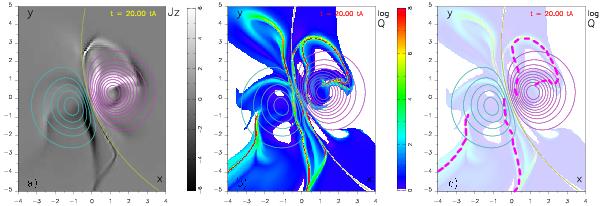
Comparison of electric currents, magnetic field, and Q distribution at z = 0. a) Plots of the photospheric current J_z (gray-scale image) and magnetic field B_z(z = 0) (cyan/pink overplotted contours for the negative/positive values, respectively). Both direct and return currents exist in the two magnetic polarities (separated by the photospheric inversion line shown in yellow). b) Logarithm of the squashing degree Q(z = 0) at t = 20  t_A showing a similar double-J structure. The color-coding for log Q is the same as in Fig. 1. c) The footprints of the main QSLs, related with the formation of the flux rope and the flare loops, are highlighted with thick dashed pink lines on top of the shaded Q-map of panel b).