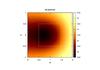
Fig. 3
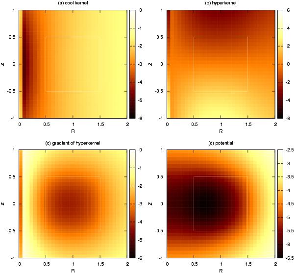
Main steps in the computation of the potential from Eqs. (25) and (27) in a typical case: a) the integral of the cool kernel, b) the integral of the hyperkernel, c) its vertical gradient, and d) the potential as the sum of maps a) and c). Here, the body is an axially symmetric torus with square cross section (boundary indicated with a white line). As clearly visible in graphs a)–c), the treatment differs slightly on the polar axis (first column of pixels). See the text for the numerical setup.
Current usage metrics show cumulative count of Article Views (full-text article views including HTML views, PDF and ePub downloads, according to the available data) and Abstracts Views on Vision4Press platform.
Data correspond to usage on the plateform after 2015. The current usage metrics is available 48-96 hours after online publication and is updated daily on week days.
Initial download of the metrics may take a while.