Free Access
Fig. 7
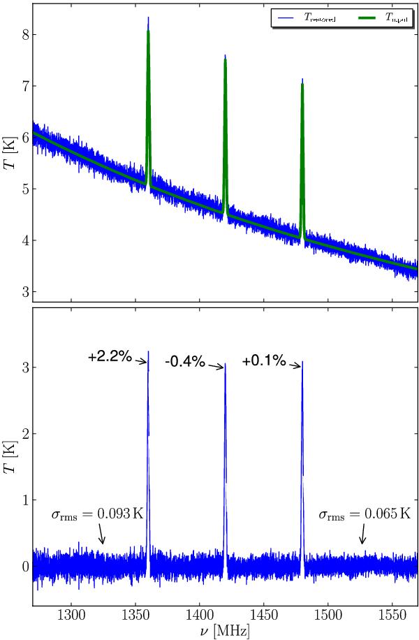
Inserting the model f [cal] (ν) into Eq. (22) results in the correct flux calibration (upper panel). The lower panel shows the spectrum after baseline subtraction. Note that the correct continuum contribution of the source was also reconstructed (upper panel). The example was computed for the SW case.
This figure is made of several images, please see below:
Current usage metrics show cumulative count of Article Views (full-text article views including HTML views, PDF and ePub downloads, according to the available data) and Abstracts Views on Vision4Press platform.
Data correspond to usage on the plateform after 2015. The current usage metrics is available 48-96 hours after online publication and is updated daily on week days.
Initial download of the metrics may take a while.