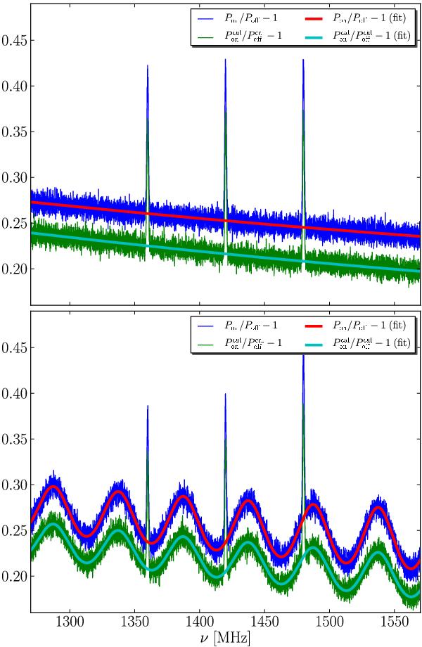
To correctly reconstruct the original fluxes, the second proposed method uses models of the intermediate spectra (see Eqs. (17) and (18)). Appropriate windows around the spectral lines should be set because one is only interested in the continuum contribution. The upper panel shows the results of the simpler case, utilising second-order polynomials sufficient to describe the baseline. For the standing wave case (lower panel), a more complicated fitting model, L₁(n₁,ν)/(L₂(n₂,ν) + Asin(aν + b)), was applied, where L_i(n_i,ν) are polynomial functions of degree n_i. In this example, we use n₁ = n₂ = 3.