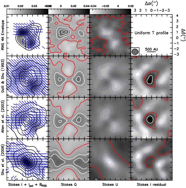
Comparison of selected models with data assuming a uniform temperature of the gas. The orientation angles are fixed to φ = 50° and ω = 45° for a better model comparison. Rows: IRAS 4A (first row); model Galli & Shu (1993a,b) with B₀ = 0.43 and τ = 0.7 (second row); model Allen et al. (2003a,b) with H₀ = 0.125, v₀ = 0 and t = 10⁴ yr (third row); and model Shu et al. (2006) with r_Ohm = 75 AU (fourth row). Columns: in each row, the panels show: intensity (first panel, contours), polarized intensity (first panel, pixel map) and magnetic field vectors (first panel, segments); map of Stokes Q (second panel, pixel map and contours); map of Stokes U (third panel, pixel and contours); residuals models-data for Stokes I (fourth panel, pixel map and contours). The color scale is shown on the top of each column. Contours: contours for the Stokes I maps (left panels) depict emission levels from 6σ up to the maximum value in steps of 6σ, where σ = 0.02 Jy beam^-1. Coutours for the Stokes Q and U maps depict levels from the minimum up to the maximum in steps of 3σ where σ = 2.5 mJy beam^-1. The solid red contour marks the zero emission level, solid white contours mark positive emission and blue dotted contours mark negative emission. Contours for the residual Stokes I follow the same rule of Stokes Q and U but with steps of 6σ, where σ = 0.02 Jy beam^-1. The top right panel shows the beam and the angular and spatial scale.