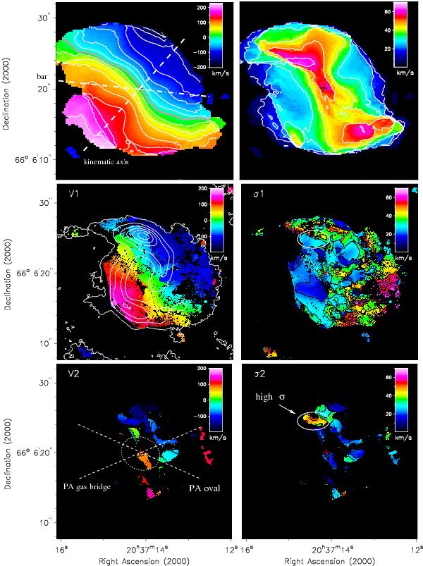
Top left: first moment map of the CO(1−0) emission. Contours: –200 to 175 km s^-1 with 50 km s^-1 steps, 0 km s^-1 thick gray contour. Kinematic major axis (white dashed line at PA = 138°), orientation of the large-scale bar (dashed-dotted line, PA = 84°). Top right: second moment map of the ¹²CO(1−0) emission. Contours: 0 to 70 km s^-1 in 10 km s^-1 steps. The dynamical center is marked by a black cross. Middle/Bottom panels: decomposed velocity field of the CO(2−1) natural weighted line emission. Black spots correspond to blanks due to bad fits at some spatial pixels. Middle left: the central value of the Gaussian fitted for each spatial pixel. If two Gaussians where fitted, the value of the Gaussian closest to the large-scale bar model velocity is given. The white contours represent the CO(2−1) intensity map (5σ in 40σ steps). Bottom left: for the spatial pixels where a double Gaussian was fitted, we plot the central value of that second Gaussian here, i.e. the value further away from the bar model velocity. The size and PA of the nuclear stellar oval and PA of the gasbridge, that will be discussed in Sect. 6.2, are highlighted with a white ellipse and dashed lines. Middle/Bottom right: velocity dispersion corresponding to respective velocity components. The dispersion is the Gaussian fitted σ at each position. Contours from 0 to 70 km s^-1. The region with significant differences in velocity dispersion (discussed in Sect. 3.3) is highlighted with a white ellipse.