| Issue |
A&A
Volume 708, April 2026
|
|
|---|---|---|
| Article Number | A271 | |
| Number of page(s) | 9 | |
| Section | Atomic, molecular, and nuclear data | |
| DOI | https://doi.org/10.1051/0004-6361/202659106 | |
| Published online | 16 April 2026 | |
Measurements and predictions of H2 pressure-broadening coefficients of CO2 absorption lines for exoplanet atmosphere studies
1
Laboratoire de Météorologie Dynamique, IPSL, Sorbonne Université, École Normale Supérieure, Université PSL, École polytechnique, Institut Polytechnique de Paris, CNRS,
Paris,
France
2
Université de Tunis, Laboratoire de Spectroscopie et Dynamique Moléculaire, École Nationale Supérieure d’Ingénieurs de Tunis,
5 Av. Taha Hussein,
1008
Tunis,
Tunisia
3
Univ Paris Est Créteil and Université Paris Cité, CNRS, LISA,
F-94010
Créteil,
France
★ Corresponding author: This email address is being protected from spambots. You need JavaScript enabled to view it.
Received:
23
January
2026
Accepted:
27
February
2026
Abstract
Accurate and comprehensive H2 pressure-induced broadening data for CO2 infrared lines over a wide temperature range are essential for modeling atmospheric opacity of exoplanets. However, available data are currently limited, some of which are affected by large uncertainties. In this work, H2 pressure-induced broadening and pressure-shift coefficients were determined at room temperature for the entire ν3 band of CO2 in the 4.3 µm spectral region using a high-resolution Fourier transform spectrometer. In addition, requantized molecular dynamics simulations of the CO2-H2 system were performed using an accurate intermolecular potential. These simulations provide theoretical predictions of H2 broadening coefficients for CO2 lines over a temperature range of 200–1000 K and for rotational quantum number up to J = 120. The predicted results show very good agreement with the experimental data, with difference of less than 3%, well below the precision required for exoplanet atmosphere studies. This work provides the first accurate and comprehensive dataset of H2 broadening coefficients for CO2 lines, suitable for modeling of H2-rich exoplanetary atmospheres.
Key words: line: profiles / molecular data / opacity / radiative transfer / methods: laboratory: molecular / techniques: spectroscopic
© The Authors 2026
 Open Access article, published by EDP Sciences, under the terms of the Creative Commons Attribution License (https://creativecommons.org/licenses/by/4.0), which permits unrestricted use, distribution, and reproduction in any medium, provided the original work is properly cited.
This article is published in open access under the Subscribe to Open model. This email address is being protected from spambots. You need JavaScript enabled to view it. to support open access publication.
1 Introduction
Reliable H2 pressure-broadening data for a variety of molecules and under wide temperature conditions are essential for accurately modeling exoplanetary atmospheres (Hedges & Madhusudhan 2016; Fortney et al. 2019; Tan et al. 2022). The accuracy of molecular abundances, or more generally atmospheric properties, derived from measured spectra depends on the precision of molecular cross sections, which relies on the knowledge of molecular spectroscopic data, including line position, line intensity, pressure-induced line broadening, and shift due to collisions between the optically active molecule and the main constituents of the considered atmosphere. Several studies demonstrated that the lack of pressure-broadening data leads to large impacts on opacity modeling and the retrieval of atmospheric properties for planets and exoplanets (e.g., Hedges & Madhusudhan 2016; Gharib-Nezhad & Line 2019; Garland & Irwin 2019; Wiesenfeld et al. 2025).
However, reliable pressure-broadening information under exoplanet thermophysical conditions remains scarce due to the wide variety of constituents, and temperature and pressure conditions that must be considered. In the absence of available experimental and theoretical data, air-broadened widths are often used with empirical scaling factors (Wilzewski et al. 2016; Tan et al. 2019, 2022) to describe the broadening by the main interfering gases in exoplanetary atmospheres such as H2 and He. This approach can cause significant discrepancies when compared to accurate measured or calculated broadening data (see Hendaoui et al. 2026, for instance). Furthermore, the temperature range encountered in exoplanet atmospheres extends far beyond that of the Earth’s atmosphere. For instance, Fortney et al. (2019) noted that for H2- and He-dominated exo-planet atmospheres, the temperature of interest spans from 70 K to 3000 K.
Carbon dioxide (CO2) is a key molecule in exoplanetary atmospheres. It is detected in a wide range of planets observed with the James Webb Space Telescope (JWST; e.g., Ahrer et al. 2023; Balmer et al. 2025). The prominent 4.3 µm absorption feature is especially valuable as it lies in a spectral region with minimal noise and cloud-haze interference, making it of great interest for both detection and habitability assessments (see Wiesenfeld et al. 2025 and references therein). Exploiting this feature is, however, limited by incomplete opacity models, particularly uncertainties in line-broadening and far-wing parameterizations (Niraula et al. 2022). Wiesenfeld et al. (2025) showed that a precision on pressure-broadening coefficients of better than 10% is required for JWST exoplanet studies.
Despite their importance, there are few studies devoted to the measurement or calculation of the H2 pressure-broadening coefficients for CO2 lines. In Padmanabhan et al. (2014), H2 broadening coefficients were measured at room temperature for ten CO2 lines, ranging from P(16) to P(34), in the 6317–6335 cm−1 region of the 30012 ← 00001 band, using a tunable diode laser. These coefficients were derived from spectra measured for mixtures of CO2, N2, and H2, with a stated uncertainty of about 6%. The measured coefficients vary significantly with the rotational quantum number, from 0.095 cm−1/atm for the P(32) line to 0.121 cm−1/atm for the P(20) line. However, no clear rotational dependence is observed, indicating that the actual uncertainty is probably larger than 6%. Hanson and Whitty (Hanson & Whitty 2014) measured the H2 broadening coefficient for the P(24) line of CO2 at 4957.08 cm−1, using wavelength-scanned spectroscopy. These measurements were taken at various temperatures, from 300 K to 700 K, with an uncertainty claimed to be better than 2%. Their room temperature value for the P(24) line is 0.112 cm−1/atm, which closely matches the value of 0.1128 cm−1/atm reported by Padmanabhan et al. (2014) for the same line. Hanson and Whitty also deduced a temperature dependence exponent of 0.582 for this P(24) line. The experimental investigation by Burch et al. (1969) suggested that H2 broadening is 1.17 times larger than self-broadening for CO2 lines, with the same rotational dependence assumed for broadening by various collision partners. These limited data have been used in various radiative transfer models to calculate the optical thickness of exoplanet atmospheres (e.g., Tremblin et al. 2015; Goyal et al. 2017; Garland & Irwin 2019).
More recently, Wiesenfeld et al. (2025) conducted ab initio calculations of H2 pressure broadening for the P(24) line of CO2 in the ground vibrational state. They found that their calculations agree with the measured values of Padmanabhan et al. (2014); Hanson & Whitty (2014) within 7%. Nie et al. (2025) measured room temperature H2 broadening coefficients for four CO2 lines in the 20012←00001 band, from R(44) to R(50) using a distributed feedback laser. H2 broadening coefficients of CO2 lines in the HITRAN database (Gordon et al. 2021) were simply obtained using a scaling factor of 1.5767 on the air-broadening coefficients. Additionally, a constant temperature dependence exponent of 0.58 was applied to all CO2 transitions in HITRAN. It is evident that more accurate and comprehensive measurements and calculations are necessary to provide more reliable line-shape data for this system.
In order to provide a reliable and comprehensive dataset for H2 broadening coefficients of CO2 lines relevant for exo-planet atmosphere studies, we conducted high-resolution laboratory measurements and first-principle calculations. Specifically, a high-resolution Fourier transform spectrometer was used to record spectra of CO2 highly diluted in H2 in the 4.3 µm spectral range, at room temperature and pressures ranging from 150 mbar to 1060 mbar. The recorded spectra were then analyzed to extract both the pressure-broadening coefficients and the pressure-induced shifts of 61 CO2 lines, from P(62) to R(60). A detailed uncertainty analysis was performed on the obtained parameters, considering uncertainties from various sources. This study represents the first measurement of these coefficients for an entire ro-vibrational band of CO2. In the second step, we used requantized classical molecular dynamics simulations (rCMDSs) to predict CO2 line broadening by H2 over a broad temperature range, from 200 K to 1000 K, which is highly relevant for opacity modeling in exoplanetary atmospheres. These simulations, based on the use of accurate intermolecular potentials and classical theory of molecular collisions, have previously demonstrated the ability to reproduce self-, air-, and He-broadened CO2 line-shape parameters (Ngo & Tran 2025; Tran et al. 2025; Hendaoui et al. 2026) with relative errors well below 5% for rotational quantum numbers up to J=160 and temperatures as high as 3000 K.
The paper is organized as follows. Section 2 focuses on the experimental determination of the pressure-induced line broadening and shift. Section 2.1 describes the experimental setup, the measurement procedure, and the determination of the instrument line shape. The fitting procedure and uncertainty analysis are detailed in Sect. 2.2. The obtained line-broadening and pressure-shift parameters are presented and compared with available data in Sect. 2.3. The rCMDS first-principle calculations for CO2–H2 are described in Sect. 3. Section 3.1 details the calculation methods and procedures. The predicted broadening coefficients are then presented and compared with measured values in Sect. 3.2, while the temperature dependence of line broadening is described in Sect. 3.3. Finally, in Sect. 4 we present the conclusions of this work.
Pressures and temperatures of the recorded spectra.
2 Measurements
2.1 Experimental setup and recording procedure
The high-resolution Fourier transform spectrometer (FTS) at LISA (Bruker IFS-125 HR) was used to record all spectra. The instrument was equipped with a silicon carbide Globar source, a KBr/Ge beamsplitter, and a liquid nitrogen cooled indium anti-monide (InSb) detector. The diameter of the FTS iris aperture was set to 2 mm and the focal length of the collimator was 418 mm. No artificial optical weighting was performed (a boxcar function was selected). A 12.3 cm simple-pass absorption cell was used. The Bruker spectral resolution was 0.01 cm−1, corresponding to a maximum optical path difference of 90 cm.
The measurements were carried out as follows. The cell was first filled with a very small quantity of CO2 (measured with a 2-Torr full-scale Baratron gauge, MKS 627D model, with an accuracy of 0.15% of reading) and then completed with H2 to reach the desired total pressure. The latter was measured with a 1000-Torr full-scale Baratron gauge, MKS 628D model, with a stated accuracy of 0.25% of reading. Commercial carbon dioxide and hydrogen samples from Air Liquide were used without purification (99.9% natural CO2; 99.9999% H2). After approximately 20 minutes, once the mixture was homogeneous, a spectrum was recorded by co-adding 3200 scans over a period of 24 hours. The cell was then pumped out and refilled to reach the next desired total pressure. This procedure was adopted to limit any leakage of ambient air into the cell during measurement. The variation in total pressure during 24-hour acquisition was approximately 0.3 mbar (with a mean leak of 2.12 10−4 mbar/min). The average temperature during the recordings was about 293.71 K, with a mean variation of 0.3 K per recording (room temperature was used as a proxy for cell temperature). In total, four spectra of mixtures with total pressure ranging from 150 mbar to 1060 mbar were recorded with spectral range spanning from 2200 cm−1 to 2500 cm−1. This spectral region covers the entire CO2 ν3 band of interest. The experimental pressures and temperatures of the recorded spectra are summarized in Table 1.
Two empty-cell spectra were recorded with the same optical conditions after pumping down to a pressure below 10−4 mbar. These provided the 100% transmission baseline by removing remaining traces of H2O and CO2 inside the interferometer, and enabled partial removal of the multiplicative channel due to interferences arising from the parallel faces of the cell windows. For each pressure, the corresponding spectrum was obtained by dividing the spectrum recorded with gas by the empty-cell spectrum. A signal-to-noise ratio up to ~1500 (see Figure 1) was achieved for the transmission spectra.
A pure CO2 spectrum at 0.08 mbar was also recorded to determine the instrument line shape (ILS) using the LINEFIT 14.8 software (Hase et al. 1999; Hase 2012). The results show small asymmetry on the ILS and a modulation close to 1, demonstrating that the different optics of the instrument were well aligned. We performed several tests to determine the optimal spectral interval and sampling step for the ILS.
For spectral calibration, we used CO2 lines appearing in the empty-cell spectra due to small residual amounts of CO2 inside the FTS. The positions of eight intense lines, determined from fits using a Gaussian profile, were compared with the corresponding line positions given in the HITRAN database (Gordon et al. 2021). The resulting calibration factor was 1.000000467, the standard deviation of the fitted positions being about 2x10⁻⁵ cm−1. As discussed below, because the contribution of weak lines is fixed in the fits using HITRAN spectroscopic line position, accurate spectral calibration is important.
It should be noted that, due to the very small quantity of CO2 introduced (see Table 1), possible partial adsorption of the gas on the cell walls, and minor leaks during gas filling, the CO2 partial pressure in the mixture is not known with high precision. However, since the absolute line intensity is not the focus of this work and because the amount of CO2 is very small, the uncertainty in the CO2 pressure does not affect the measured H2 pressure-induced line shape of the considered CO2 transitions.
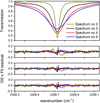 |
Fig. 1 Measured transmission of the R(12) line (top panel) and fit residuals obtained by fitting the measured spectra with the Voigt profile (second panel), with LM accounted for (third panel) and with the HC model together with LM (bottom panel). |
2.2 Spectra analysis and uncertainty determination
The measured transmission spectrum of CO2 broadened by H2 can be expressed as:
![Mathematical equation: $\matrix{ {} \hfill & {T\left( {\sigma ,{P_{C{O_2}}},{P_{{{\rm{H}}_2}}},T} \right)} \hfill \cr {} \hfill & {\quad = \exp \left[ { - L{P_{{\rm{C}}{{\rm{O}}_2}}}\mathop \sum \limits_i {S_i}(T)\phi \left( {\sigma - {\sigma _i},{P_{{\rm{C}}{{\rm{O}}_{\rm{2}}}}},{P_{{{\rm{H}}_2}}},T} \right)} \right] \otimes {\rm{ILS}}} \hfill \cr } $](/articles/aa/full_html/2026/04/aa59106-26/aa59106-26-eq1.png) (1)
(1)
where the symbol ⊗ indicates the convolution between the high-resolution transmission with the instrument line-shape function, L (cm) is the absorption path length, and  and
and  (atm) are respectively the CO2 and H2 pressures in the mixture. The sum is over all lines contributing to absorption at wavenumber σ (cm−1). The quantity Si (T) (cm−2 atm−1) is the intensity of the line i at temperature T (K) and ϕ(σ − σi,
  ,
,  , T) (in cm) is the line shape or the normalized profile of this line. In the simplest case, this line-shape function is expressed by the Voigt profile, which is a convolution of a Gaussian and a Lorentzian profile, taking into account respectively the Doppler broadening and pressure-induced broadening and shift of the line. More sophisticated models can be used for ϕ as well, taking into account more refined pressure-induced collisional effects such as the speed dependence of the line broadening and shift, the Dicke narrowing, and the collision-induced interferences between line (i.e., line mixing) (Ngo et al. 2013; Wcisło et al. 2025).
Here we used three different profiles to fit the measured spectra: the usual Voigt profile, the Voigt profile with line mixing (LM) accounted for, and the hard-collision (HC) profile with LM. The Doppler width was calculated for the temperature of the measurement of each spectrum and fixed in the fits. For the Voigt profile, two line-shape parameters were fitted: the H2 pressure-broadening coefficient,  , and the H2 pressure shift,
  (both in cm−1/atm). To model the weak LM effects between CO2 lines at the considered pressures, we used the first-order approximation (Rosenkranz 1975). In this case, the LM coefficient, ξ (atm−1), is also adjusted. Finally, to model the weak Dicke narrowing effect, due to molecule velocity changes caused by collisions, we used the hard-collision model (Nelkin & Ghatak 1964), leading to an additional parameter to be fitted, the Dicke narrowing parameter, or the velocity changing rate, νVC (cm−1/atm). When the signal-to-noise ratio of the measured spectra is high enough, refined line-shape models lead to better agreement with measurements. The retrieved line-broadening coefficient also slightly depends on the used line shapes (see Ngo et al. 2013 and references therein).
A multi-fitting procedure was used, in which we fitted simultaneously the four measured spectra of CO2 in H2, constraining the different line-shape parameters (i.e.,  ,
,  , ξ, and νVC) to be the same at different pressures. The instrument line-shape function, determined from the pure CO2 spectrum measured at low pressure, as explained in Sect. 2.1, was fixed in the fits. In addition to the line-shape parameters, the line area [i.e.,
  (T)] and line position (at zero pressure) were also fitted. Spectral ranges about 2 cm−1 were considered at a time in the fits. All lines with integrated intensity greater than 1 × 10⁻²⁰ cm−1/(molec · cm−2) were fitted. These correspond to lines of the ν3 band of the main isotopologue of CO2 with rotational quantum number J up to 62. The contribution of weaker lines was calculated for the measured experimental conditions using spectroscopic data from the HITRAN database (Gordon et al. 2021), except for the line broadening coefficient. The latter was estimated from the first round fits of the ν3 lines of 12CO2 and neglecting any vibrational and isotopic dependences of the broadening coefficient. For the calculation of weak lines, the partial pressures of CO2 for each spectrum was redetermined using the fitted areas and integrated intensities in HITRAN for several strong ν3 lines of 12CO2. For each spectral range and pressure, we used two baseline models for the 100% transmission: a linear baseline and a third-order polynomial function. The parameters of the baseline were also fitted. The difference in the retrieved line-shape parameters obtained with these two baseline models was accounted for in the estimation of their uncertainties.
Examples of the measured transmissions and the corresponding fit residuals obtained with the three line-shape models are shown in Fig. 1. The residuals obtained with LM taken into account are close to the experimental noise level; the weak remaining residuals are probably due to the imperfect modeling of the instrument line shape. It was not possible to fit all lines with the HC model with first-order LM, probably due to the limited signal-to-noise ratio of the measured spectra. This model resulted in only marginally better fit residuals compared to those obtained with the Voigt model with LM. In addition, the differences between the  values obtained with Voigt+LM and HC+LM are well below the total uncertainty. We note that a similar conclusion was obtained when using the speed-dependent Voigt profile (Ngo et al. 2013) to fit the measured spectra. Therefore, in the following, we focus and discuss results obtained with Voigt+LM only.
The uncertainty of the fitted parameters comes from different sources. The first is the statistical uncertainty (type A), corresponding to the standard deviation obtained from the fits. This quantity is negligibly small compared to the systematic uncertainties. The latter arise from the uncertainty in the measured pressure and temperature, and in the apparatus function. In our analysis, we assumed that self-broadening effects are the same as H2 broadening effects, i.e.,  . This assumption has a largely negligible effect on the determined H2 collision-induced line-shape parameters since the concentrations of CO2 in the mixtures are low (see Table 1). To determine the uncertainty due to errors in the measured Ptot, we reanalyzed the four measured spectra, but with the total pressure
  , where ∆P is the error in the measured total pressure. The corresponding uncertainty of the line-shape parameters was then determined as the difference between the parameters obtained using
  and those obtained using
  . A similar procedure was performed to determine the uncertainty due to the uncertainty of the measured temperature. In addition, the line-shape parameters were considered as being obtained at the average temperature. The uncertainty due to the difference between the average temperature and the temperature measured for each spectrum was also considered, using the temperature dependence exponent of H2 broadening coefficients provided in the HITRAN database (Gordon et al. 2021). Uncertainties due to errors in the ILS were estimated by performing fits with two ILSs, both determined using LINEFIT, by applying LINEFIT to selected microwindows and to the entire R branch in the pure CO2 spectrum. The total uncertainty for each retrieved parameter was then computed as the sum of all individual contributions, including that arising from the choice of baseline models. Except for a few lines of high rotational quantum number, this computed uncertainty is below 2%. We therefore assume that the total uncertainty of the measured
  for these lines is 2%.
2.3 Results and comparison with available data
The obtained values of  are listed in Table 2, and are plotted in Fig. 2 as a function of |m|, where m = –J and m = J+1 in the P and R branches, respectively. The data available in the literature are also displayed in Fig. 2 for comparison. As can be observed, for the P(24) line, our result is in very good agreement with that of Hanson & Whitty (2014), with a difference of 0.25%. The calculated value of Wiesenfeld et al. (2025) for the same line is about 9% larger than our result. Larger discrepancies, up to 15%, are observed when comparing our values with those of Padmanabhan et al. (2014). In the latter study, a large and apparently random variation of
  with |m| is observed, which is not the case for our data. Differences of up to 9% and 5% are observed when comparing our results with those of Nie et al. (2025) obtained with the Voigt and the HC profiles, respectively. We note that Nie et al. (2025) determined line intensity and broadening coefficients from spectra measured for mixtures of CO2 with various perturbers such as O2, N2, H2, and Ar. Their retrieved line intensity depends strongly on the perturber, with variation up to 3.2%, indicating large uncertainty in the retrieved parameters. Therefore, the actual uncertainty in the measured broadening must be significantly larger than the 1% uncertainty claimed. Finally, significant differences of up to 16.5% are also found when comparing our results with the values provided in HITRAN (Tan et al. 2022). The
  values in HITRAN were obtained by simply scaling the air-broadening coefficient to match the results of Hanson & Whitty (2014) at |m| = 24 (Tan et al. 2022). Our results therefore demonstrate that the rotational dependence of
  differs significantly from that of γair. Consequently, using these data (Padmanabhan et al. 2014; Tan et al. 2022) for opacity modeling of planetary and exoplanetary atmospheres may lead to substantial errors.
The measured pressure-shift coefficients,  , are plotted in Fig. 3 versus the rotational quantum number. This work provides the first determination of
  for the ν3 band. It is important to emphasize that
  were obtained by fitting the measured spectra accounting for LM effects. When a simple Voigt profile is used (neglecting LM), the derived coefficients differ significantly and exhibit a strong rotational dependence (see Fig. 3). This behavior is due to the influence of line-mixing effects, which can shift the peak absorption. As can be seen, the rotational dependence of
  is weak, similarly to what was observed for CO2 broadened by He (Hendaoui et al. 2026), although the magnitude of
  is significantly larger. The mean value of
  is –3.9 10−3 cm−1/atm, compared to –0.52 10−3 cm−1/atm for He. To the best of our knowledge, the only previously available data on
  are those reported by Nie et al. (2025). In that study, H2 pressure-induced shifts were measured for four CO2 lines in the ν1 + 2ν2 + ν3 band, yielding a mean value of about – 7.5 10−3 cm−1/atm. The difference between their result and the present measurements can be attributed to the strong vibrational dependence of the pressure-induced line shift.
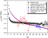 |
Fig. 2 H2 broadening coefficient measured in this work, and a comparison with the available experimental and theoretical data and with the values from HITRAN (Tan et al. 2022). |
H2 pressure-broadening and pressure-shift coefficients of CO2 lines in the ν3 band measured around 294 K.
 |
Fig. 3 H2 pressure shift determined from fits of measured spectra with the Voigt profile (without LM) and with LM taken into account. |
3 Theoretical predictions of 
3.1 Calculation method and data used
We employed rCMDSs to predict  over a broad temperature range, from 200 K to 1000 K. Using accurate intermolecular potentials and the Newtonian equations of motion, this method enables the simulation of the time evolution of a system containing a large number of molecules at a given pressure and temperature (Allen & Tildesley 1987). The auto-correlation functions (ACFs) of the dipole moment, responsible for the transitions, can thus be computed. The Fourier–Laplace transform of these ACFs directly yields the spectral density or the normalized spectral profile. In addition, we applied a requantization procedure (Hartmann et al. 2013) to the molecular rotation. The requantized spectral line obtained this way can then be fitted with a line-shape model, such as the usual Voigt profile, to deduce the corresponding pressure broadening. This approach has enabled very satisfactory predictions of line-shape parameters (Nguyen et al. 2018; Tran et al. 2019; Nguyen et al. 2020; Ngo et al. 2021; Hendaoui et al. 2024; Ngo & Tran 2025; Tran et al. 2025; Hendaoui et al. 2026), far-wing absorption (Hartmann et al. 2010, 2018), and collision-induced absorption (Hartmann & Boulet 2011; Hartmann et al. 2017; Fakhardji et al. 2022) for various molecular systems and under wide ranges of pressure and temperature.
At the initial time, the molecules were positioned as follows: the center of mass of each molecule was randomly assigned, with a minimum separation of 7 Å to prevent unphysically strong interactions. The system then reaches equilibrium after a temperature- and pressure-dependent temporization time, ttempo. Translational and angular speeds were initialized according to Maxwell–Boltzmann distributions, with random velocity vectors and molecular axis orientation assigned to each molecule. At each time step, the forces and torques acting on each molecule were computed to update their accelerations, translational velocities, position, angular velocities, and molecular orientations at the next time step t + ∆t.
A requantization procedure (Hartmann et al. 2013) was applied to the classical rotation of the CO2 molecules, but only when the interaction between the considered CO2 molecule and its neighboring H2 molecules was negligible. This approach, well suited for the CO2 molecule due to the small energy separation between its rotational levels, was shown to yield excellent predictions of CO2 broadening coefficients in N2, O2, He and self-broadening (Nguyen et al. 2018, 2020; Ngo & Tran 2025; Hendaoui et al. 2026). Specifically, for a molecule of rotational angular speed ω, the even integer J is determined such that  is closest to ω, where I is the moment of inertia. This procedure matches the classical rotational frequency with the quantum position of the P-branch lines. Once J is found, ω is requantized by applying the change
  , while the orientation of the rotational angular momentum remains unchanged. This P-branch requantization implies that the R-branch will be an exact mirror image of the P-branch.
The ACF of the dipole moment vector, assumed along the CO2 molecular axis (as is the case for the asymmetric stretching absorption bands of CO2), was then calculated during the rCMDSs. The Doppler effect associated with the translational motion was also included. Finally, the spectral profile (or the normalized absorption coefficient) was obtained from the Fourier– Laplace transform of the dipole moment ACF (Hartmann et al. 2021).
Here CO2 molecules were modeled as linear rigid rotors in their equilibrium configuration, with all effects of vibrational motion disregarded in the calculations. This approximation is expected to have a negligible effect on the calculated pressure broadening (Hashemi et al. 2020). The CO2-H2 interaction was described using the site-site potential provided by Hellmann & Bich (2025). The parameters of this site-site potential, as well as the positions of the sites in the molecules were determined from the ab initio calculated interaction energies as described in Hellmann & Bich (2025). The spectra were thus calculated without using any parameter adjusted to the experimental data. We note that our rCMDSs do not account for dipole dephasing, which arises from different intermolecular interactions in the upper and lower states of the transitions. As a result, the calculated spectra do not show any pressure-induced vibrational shifts.
The simulations were performed on the Jean-Zay HPE SGI 8600 supercomputer at the Institut du Dévéloppement et des Ressources en Informatique Scientifique, which supports massively parallel computing. The molecules were distributed across four thousand boxes with periodic boundary conditions (Allen & Tildesley 1987), each containing 20 000 molecules. Mixtures containing 50% CO2 were considered, but only CO2-H2 interactions were accounted for. This is equivalent to CO2 being infinitely diluted in H2, with the total pressure corresponding to the partial pressure of H2. rCMDSs were performed for the following temperatures: 200 K, 296 K, 400 K, 500 K, 600 K, 800 K, and 1000 K. For each temperature, the pressure of the mixture was chosen such that line-mixing effects were negligible (pressures up to 0.5 atm for T ≤ 400 K and up to 1 atm for T between 500 K and 1000 K). For each temperature, a total number of 8 × 10⁷ molecules was considered, yielding signal-to-noise ratios of the calculated spectra of up to 1000 for the most intense lines.
Spectra calculated with rCMDS were fitted with Voigt profiles to retrieve the pressure-broadening coefficients. The line position, line area, and a linear baseline were also fitted, as for the measured spectra. Additional fits were performed using more refined models, such as the speed-dependent Voigt and HC profiles, to account for the speed dependence of line broadening and for Dicke narrowing, respectively. However, the results show that these effects have a negligible influence on the fit residuals and on the retrieved line-broadening coefficients. The pressure-broadening coefficients obtained from the rCMDS-calculated spectra at all considered temperatures are presented and compared with the experimental values in the next subsection.
 |
Fig. 4 H2 broadening coefficient predicted by rCMDS at 296 K, and a comparison with the experimental values of the present work and with the HITRAN data. The gray space represents the 10% precision level required for exoplanetary atmosphere studies. |
3.2 H2 broadening coefficient predicted by rCMDS
Figure 4 shows the broadening coefficients obtained from rCMDS at 296 K and their comparison with our accurate experimental values, where a very good agreement can be observed. Except for the P(2) line, for which a difference of 4% is observed, the discrepancies between the rCMDS predictions and the measured values are well below the experimental uncertainty (2%). We note that, for this comparison, the measured values were converted to 296 K using a single power law and the associated temperature dependence obtained from rCMDS, as listed in Appendix A. This level of agreement is significantly better than the precision of 10% required for opacity calculations in exoplanet studies with JWST (Wiesenfeld et al. 2025). In contrast, the current HITRAN data (red curve in Fig. 4, (Tan et al. 2022)) leads to substantial deviations of up to 16.5% relative to the rCMDS values. The comparison presented in Fig. 4 therefore fully confirms the validity of our rCMDS method for predicting H2 broadening coefficient of CO2 lines.
rCMDS calculations were performed for six additional temperatures: 200 K, 400 K, 500 K, 600 K, 800 K, and 1000 K. For each temperature,  was carefully determined for all considered lines. As the number of populated rotational levels increases with temperature,
  was determined up to a maximum rotational quantum number J = 50 at 200 K, while at 1000 K line broadening was obtained for lines up to J = 120. Figure 5 presents the rCMDS-predicted results at 600 K and 1000 K, together with corresponding
  values from HITRAN (Tan et al. 2022). Large discrepancies are observed at all temperatures, with deviations reaching more than 30%.
At 600 K, our results are also compared with the experimental measurements of Hanson & Whitty (2014), who measured the H2 broadening coefficient for the P(24) line and provided a temperature dependence exponent of 0.582. The value calculated by Wiesenfeld et al. (2025) at 600 K for the same line is also shown. As illustrated in Fig. 5, our rCMDS results are about 10% smaller than those of Hanson & Whitty (2014) and Wiesenfeld et al. (2025). Nevertheless, given the excellent agreement between rCMDS predictions and accurate experimental data at room temperature (Fig. 4), as well as the improved validity of classical treatment for molecular rotations at higher temperatures, we are confident in the reliability of our results. Additional accurate measurements of H2 broadening coefficients at temperatures above room temperature would nevertheless be valuable for further validation.
As can be seen in Figs. 4, 5, a noticeable scatter is present in the rCMDS-predicted broadening coefficients, particularly for high |m| values. This scatter mainly arises from the lower signal-to-noise ratio of the corresponding lines, which leads to increased uncertainty in the extracted line broadening. To mitigate this effect, the rCMDS-predicted broadening coefficients at each temperature were fitted using a Padé approximant, as was done in Tan et al. (2022); Hendaoui et al. (2026). As illustrated by the examples in Fig. 5, the quality of these fits is excellent. The fitted functions were then used to deduce broadening coefficients for R-branch lines, assuming symmetry between P- and R-branch coefficients with respect to m. This symmetry assumption has a negligible impact on the collisional line broadening of CO2 (Mondelain et al. 2025). In addition, as  tends toward a constant value at high J (see Figs. 4, 5), these functions can be safely used to extrapolate
  for J up to 120 for all considered temperatures. The fitted broadening coefficients were then used to determine their temperature dependence, which is presented in the following subsection.
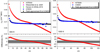 |
Fig. 5 H2 broadening coefficient predicted by rCMDS at 600 K and 1000 K, and a comparison with values of HITRAN (Tan et al. 2022). The gray space represents the 10% precision level required for exoplanetary atmosphere studies. |
3.3 Temperature dependence
We used both the usual single power law (SPL) and the recently recommended double power law (Gamache & Vispoel 2018) (DPL) to model the temperature dependence of  . In the SPL, the temperature dependence of
  is expressed as
 (2)
(2)
with T0 = 296 K and n the temperature-dependence exponent. In the DPL,  is written as
 (3)
(3)
For each transition, both the SPL and DPL were fitted to the rCMDS-predicted values of  at six temperatures: 200 K, 296 K, 400 K, 600 K, 800 K, and 1000 K. In the SPL fits the parameters
  and n were fitted, while in the DPL four parameters γ0,
  , n1 and n2 were fitted.
Figure 6 presents examples of fits with the SPL and DPL for the P(8) and R(28) lines. The corresponding differences between the rCMDS results and the fitted broadenings are also shown. As can be observed, the DPL provides better overall agreement with rCMDS predictions, with deviations always below 1%, whereas the SPL leads to discrepancies of up to 4%, especially at high temperatures.
Examples of the fitted parameters ( , n, γ0,
  , n1, and n2), together with their standard deviations are reported in Appendix A, while the results for all considered lines are available on the Zenodo platform at the following link: https://zenodo.org/records/18350127. To further verify the quality of the fits, we recalculated
  using both the SPL and DPL parameterizations and compared the results with direct rCMDS predictions at 500 K. The results show very good agreement, with maximum deviations of 3% for the SPL and 1% for the DPL.
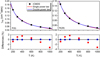 |
Fig. 6 rCMDS-predicted H2 broadening coefficients vs. temperature (black squares) for two lines P(8) and R(28), and their fits using a single power function (red line) and a double power function (blue line). The differences between the rCMDS values and fits are displayed in the corresponding lower panels. |
4 Conclusions
Accurate and comprehensive H2 broadening coefficients for CO2 lines under a wide temperature range are necessary for reliable opacity modeling of exoplanetary atmospheres. In this work, we reported the first accurate measurements at room temperature of H2 broadening and pressure-shift coefficients for the entire CO2 band at 4.3 µm, obtained using a high-resolution Fourier transform spectrometer. The commonly used data derived from air-broadening coefficients scaled by a constant factor show significant discrepancies, up to 16.5%, compared to the measured coefficients.
In addition, we performed first-principle calculations based on requantized classical molecular dynamics simulations (rCMDSs) to predict H2 broadening coefficients of CO2 lines over a wide temperature range, from 200 K to 1000 K. The predicted values are in very good agreement with the experimental measurements; the maximum differences are well below 3%, thus satisfying the precision requirements for JWST exoplanet studies. The experimentally validated rCMDS results were then used to derive the temperature dependence of the line broadening.
The obtained dataset allows the calculations of H2 broadening coefficients for CO2 lines with rotational quantum number up to 120 at any temperature within the 200–1000 K range. These results are expected to significantly improve the accuracy of opacity calculation for H2-rich atmosphere exoplanets.
Data availability
The complete dataset produced in this work are accessible at the following Zenodo link: https://zenodo.org/records/18350127.
Acknowledgements
This work was granted access to the HPC resources of IDRIS under the allocation 2025-[A0180914906] made by GENCI. It was also supported by the Programme National de Planétologie (PNP) of CNRS-INSU co-funded by CNES.
References
- Ahrer, E.-M., Alderson, L., Batalha, N. M., et al. 2023, Nature, 614, 649 [NASA ADS] [CrossRef] [Google Scholar]
- Allen, M. P., & Tildesley, D. J. 1987, Computer Simulation of Liquids (Oxford: Oxford University Press) [Google Scholar]
- Balmer, W. O., Kammerer, J., Pueyo, L., et al. 2025, Astron. J., 169, 209 [Google Scholar]
- Burch, D. E., Gryvnak, D. A., Patty, R. R., & Bartky, C. E. 1969, J. Opt. Soc. Am., 59, 267 [NASA ADS] [CrossRef] [Google Scholar]
- Fakhardji, W., Boulet, C., Tran, H., & Hartmann, J.-M. 2022, J. Quant. Spectrosc. Radiat. Transf., 283, 108148 [Google Scholar]
- Fortney, J. J., Robinson, T. D., Domagal-Goldman, S., et al. 2019, arXiv e-prints [arXiv:1905.07064] [Google Scholar]
- Gamache, R. R., & Vispoel, B. 2018, J. Quant. Spectrosc. Radiat. Transf., 217, 440 [Google Scholar]
- Garland, R., & Irwin, P. G. 2019, arXiv e-prints [arXiv:1903.03997] [Google Scholar]
- Gharib-Nezhad, E., & Line, M. R. 2019, ApJ, 872, 27 [NASA ADS] [CrossRef] [Google Scholar]
- Gordon, I. E., Rothman, L. S., Hargreaves, R. J., et al. 2021, J. Quant. Spectrosc. Radiat. Transf., 107949 [Google Scholar]
- Goyal, J. M., Mayne, N., Sing, D. K., et al. 2017, MNRAS, 474, 5158 [Google Scholar]
- Hanson, R., & Whitty, K. 2014, Tunable Diode Laser Sensors to Monitor Temperature and Gas Composition in High-Temperature Coal Gasifiers, Tech. rep., Stanford Univ., CA, USA [Google Scholar]
- Hartmann, J.-M., & Boulet, C. 2011, J. Chem. Phys., 134, 184312 [Google Scholar]
- Hartmann, J.-M., Boulet, C., Tran, H., & Nguyen, M. T. 2010, J. Chem. Phys., 133, 144313 [Google Scholar]
- Hartmann, J.-M., Tran, H., Ngo, N. H., et al. 2013, Phys. Rev. A, 87, 013403 [Google Scholar]
- Hartmann, J.-M., Boulet, C., & Toon, G. C. 2017, Geophys. Res. Atmos., 122, 2419 [Google Scholar]
- Hartmann, J.-M., Boulet, C., Tran, D. D., Tran, H., & Baranov, Y. 2018, J. Chem. Phys., 148, 054304 [Google Scholar]
- Hartmann, J., Boulet, C., & Robert, D. 2021, Collisional Effects on Molecular Spectra: Laboratory Experiments and Models, Consequences for Applications (Elsevier) [Google Scholar]
- Hase, F. 2012, Atmos. Meas. Tech., 5, 603 [Google Scholar]
- Hase, F., Blumenstock, T., & Paton-Walsh, C. 1999, Appl. Opt., 38, 3417 [Google Scholar]
- Hashemi, R., Gordon, I. E., Tran, H., et al. 2020, J. Quant. Spectrosc. Radiat. Transf., 256, 107283 [Google Scholar]
- Hedges, C., & Madhusudhan, N. 2016, MNRAS, 458, 1427 [Google Scholar]
- Hellmann, R., & Bich, E. 2025, Int. J. Thermophys., 46, 67 [Google Scholar]
- Hendaoui, F., Hartmann, J.-M., Aroui, H., & Tran, H. 2026, Icarus, 445, 116861 [Google Scholar]
- Hendaoui, F., Nguyen, H., Aroui, H., Ngo, N., & Tran, H. 2024, J. Quant. Spectrosc. Radiat. Transf., 319, 108954 [Google Scholar]
- Mondelain, D., Campargue, A., Gamache, R. R., et al. 2025, J. Quant. Spectrosc. Radiat. Transf., 333, 109271 [Google Scholar]
- Nelkin, M., & Ghatak, A. 1964, Phys. Rev., 135, A4 [Google Scholar]
- Ngo, N., Nguyen, H., Le, M., & Tran, H. 2021, J. Quant. Spectrosc. Radiat. Transf., 267, 107607 [Google Scholar]
- Ngo, N., & Tran, H. 2025, J. Quant. Spectrosc. Radiat. Transf., 331, 109264 [Google Scholar]
- Ngo, N. H., Lisak, D., Tran, H., & Hartmann, J. M. 2013, J. Quant. Spectrosc. Radiat. Transf., 129, 89 [Google Scholar]
- Nguyen, H. T., Ngo, N. H., & Tran, H. 2018, J. Chem. Phys., 149, 224301 [Google Scholar]
- Nguyen, H., Ngo, N., & Tran, H. 2020, J. Quant. Spectrosc. Radiat. Transf., 242, 106729 [Google Scholar]
- Nie, W., Zhou, Z., Xu, Z., et al. 2025, Spectrochim. Acta A Mol. Biomol. Spectrosc., 328, 125428 [Google Scholar]
- Niraula, P., de Wit, J., Gordon, I. E., et al. 2022, Nat. Astron, 6, 1287 [Google Scholar]
- Padmanabhan, A., Tzanetakis, T., Chanda, A., & Thomson, M. 2014, J. Quant. Spectrosc. Radiat. Transf., 133, 81 [Google Scholar]
- Rosenkranz, P. 1975, IEEE Trans. Antennas Propag., 23, 498 [Google Scholar]
- Tan, Y., Kochanov, R. V., Rothman, L. S., & Gordon, I. E. 2019, Geophys. Res. Atmos., 124, 11580 [Google Scholar]
- Tan, Y., Skinner, F. M., Samuels, S., et al. 2022, ApJSS, 262, 40 [Google Scholar]
- Tran, D., Sironneau, V., Hodges, J., et al. 2019, J. Quant. Spectrosc. Radiat. Transf., 222, 108 [Google Scholar]
- Tran, H., Denis, L., Lepère, M., Vispoel, B., & Ngo, N. 2025, J. Quant. Spectrosc. Radiat. Transf., 342, 109499 [Google Scholar]
- Tremblin, P., Amundsen, D. S., Mourier, P., et al. 2015, ApJ, 804, L17 [CrossRef] [Google Scholar]
- Wcisło, P., Stolarczyk, N., Słowiński, M., et al. 2025, J. Quant. Spectrosc. Radiat. Transf., 347, 109596 [Google Scholar]
- Wiesenfeld, L., Niraula, P., de Wit, J., et al. 2025, ApJ, 981, 148 [Google Scholar]
- Wilzewski, J. S., Gordon, I. E., Kochanov, R. V., Hill, C., & Rothman, L. S. 2016, J. Quant. Spectrosc. Radiat. Transf., 168, 193 [Google Scholar]
Appendix A Additional table
Sample of parameters obtained from fits of the single power and double power laws to rCMDS results.
All Tables
H2 pressure-broadening and pressure-shift coefficients of CO2 lines in the ν3 band measured around 294 K.
Sample of parameters obtained from fits of the single power and double power laws to rCMDS results.
All Figures
|
Fig. 1 Measured transmission of the R(12) line (top panel) and fit residuals obtained by fitting the measured spectra with the Voigt profile (second panel), with LM accounted for (third panel) and with the HC model together with LM (bottom panel). |
| In the text | |
|
Fig. 2 H2 broadening coefficient measured in this work, and a comparison with the available experimental and theoretical data and with the values from HITRAN (Tan et al. 2022). |
| In the text | |
|
Fig. 3 H2 pressure shift determined from fits of measured spectra with the Voigt profile (without LM) and with LM taken into account. |
| In the text | |
|
Fig. 4 H2 broadening coefficient predicted by rCMDS at 296 K, and a comparison with the experimental values of the present work and with the HITRAN data. The gray space represents the 10% precision level required for exoplanetary atmosphere studies. |
| In the text | |
|
Fig. 5 H2 broadening coefficient predicted by rCMDS at 600 K and 1000 K, and a comparison with values of HITRAN (Tan et al. 2022). The gray space represents the 10% precision level required for exoplanetary atmosphere studies. |
| In the text | |
|
Fig. 6 rCMDS-predicted H2 broadening coefficients vs. temperature (black squares) for two lines P(8) and R(28), and their fits using a single power function (red line) and a double power function (blue line). The differences between the rCMDS values and fits are displayed in the corresponding lower panels. |
| In the text | |
Current usage metrics show cumulative count of Article Views (full-text article views including HTML views, PDF and ePub downloads, according to the available data) and Abstracts Views on Vision4Press platform.
Data correspond to usage on the plateform after 2015. The current usage metrics is available 48-96 hours after online publication and is updated daily on week days.
Initial download of the metrics may take a while.