| Issue |
A&A
Volume 691, November 2024
|
|
|---|---|---|
| Article Number | A246 | |
| Number of page(s) | 9 | |
| Section | Astronomical instrumentation | |
| DOI | https://doi.org/10.1051/0004-6361/202451919 | |
| Published online | 15 November 2024 | |
An optimization method for deformable mirror configuration in multi-conjugate adaptive optics systems
1
National Laboratory on Adaptive Optics,
Chengdu
610209,
Sichuan,
China
2
Institute of Optics and Electronics, Chinese Academy of Sciences,
Chengdu
610209,
Sichuan,
China
3
University of Chinese Academy of Sciences,
Beijing
100049,
China
4
School of Electronic, Electrical and Communication Engineering, University of Chinese Academy of Sciences,
Beijing
100049,
China
★ Corresponding author; This email address is being protected from spambots. You need JavaScript enabled to view it.
Received:
19
August
2024
Accepted:
10
October
2024
Abstract
Context. Multi-conjugate adaptive optics (MCAO) is a crucial technology for achieving high-resolution imaging over a wide field of view with modern ground-based optical telescopes. The configuration of deformable mirrors (DMs) is a key component in the analysis and optimization of MCAO performance. Currently, the search for the optimal DM configuration often relies on iterative and time-consuming Monte Carlo simulations. This issue arises from the lack of an appropriate optimization method for DM configurations.
Aims. The primary objective of this paper is to establish an optimization method for DM configurations in MCAO systems. We established a quantitative criterion for evaluating DM configurations by analyzing their correction capabilities for turbulence aberrations at different altitudes. Then, we optimized the DM configurations based on this criterion. This method provides a new theoretical foundation and practical tool for the design and performance optimization of MCAO systems.
Methods. Based on the pupil phase structure function, we established a DM configuration evaluation criterion, namely the non-conjugate correction index (NCCI). Using NCCI as the optimal criterion, combined with the particle swarm optimization algorithm, we searched for the optimal solution across different DM configuration spaces.
Results. We conducted simulations based on the turbulence profiles of typical telescope sites. We validated our proposed theoretical model against Monte Carlo simulation models and find that the NCCI error ranges from 0.05 to 0.1. For optimizing DM conjugate heights, the results of our optimization algorithm differ by less than 1 km from those obtained via Monte Carlo simulations. Regarding the performance of the DM optimization algorithm, the average convergence accuracy error is less than 0.1 km, and the average convergence speed is approximately ten iterations. Additionally, our optimization method runs in just a few minutes; Monte Carlo simulations, in comparison, require several dozen hours.
Key words: instrumentation: adaptive optics / methods: analytical / techniques: high angular resolution / telescopes
© The Authors 2024
 Open Access article, published by EDP Sciences, under the terms of the Creative Commons Attribution License (https://creativecommons.org/licenses/by/4.0), which permits unrestricted use, distribution, and reproduction in any medium, provided the original work is properly cited.
This article is published in open access under the Subscribe to Open model. This email address is being protected from spambots. You need JavaScript enabled to view it. to support open access publication.
1 Introduction
Multi-conjugate adaptive optics (MCAO) is a critical technology for modern ground-based optical telescopes to achieve high-resolution imaging over a wide field of view (FOV; Zhang et al. 2023, 2024; Rao et al. 2024; Rigaut & Neichel 2018). The fundamental principle of MCAO involves using multiple wavefront sensors to detect cumulative wavefront distortions from different guide star (GS) directions. A tomographic algorithm is then employed to reconstruct the atmospheric turbulence, thereby obtaining wavefront distortions at different altitudes of the turbulent layers. These reconstructed wavefronts are subsequently projected onto multiple deformable mirrors (DMs) to compensate for these distortions (Fusco et al. 2001), thus carrying out a three-dimensional detection and correction process for atmospheric turbulence (Ragazzoni et al. 1999; Beckers 2000). Due to the comprehensive detection and compensation of atmospheric turbulence through tomographic reconstruction and layered correction, MCAO is capable of achieving higher image quality over a larger corrected FOV, addressing the narrow correction field issue present in conventional adaptive optics (AO; Beckers 1989; Fusco et al. 2005). Currently, the MCAO systems have been or are planned to be implemented in various telescopes to enhance their observational capabilities, including the Daniel K. Inouye Solar Telescope (DKIST; Schmidt et al. 2022), the European Solar Telescope (EST; Noda et al. 2022), and night-time astronomical telescopes such as the Very Large Telescope (VLT; Marchetti et al. 2007; Rigaut et al. 2021), the Extremely Large Telescope (ELT; Ciliegi et al. 2024), the Thirty Meter Telescope (TMT; Crane et al. 2018), and so on.
In the design of an MCAO system, the configuration of DMs, including their number and conjugate heights, typically depends on the characteristics of the turbulence distribution at the telescope site. The range of possible DMs is limited: too few will result in insufficient compensation for wavefront distortions caused by turbulence layers, making it difficult to achieve high-resolution imaging, while too many will increase the complexity of both the algorithms and the system (Fusco et al. 1999). Regarding conjugate heights (Tokovinin et al. 2000), although MCAO aims to correct aberrations from turbulence layers at different altitudes, DMs positioned at various conjugate heights often cannot completely correct wavefront disturbances from all turbulence layers. Uncorrected turbulence layers can significantly increase system correction errors, lim-iting both the correction FOV and the imaging quality of the MCAO system. For well-established MCAO systems like Gemini (Boccas et al. 2008), Multi-conjugate Adaptive Optics Demonstrator (MAD; Marchetti et al. 2003), and Goode Solar Telescope (GST; Schmidt et al. 2017), determining the optimal DM configuration typically requires many Monte Carlo simulations in the early stages of a project. Thus, the configuration of DMs directly impacts the correction of turbulence layers at different heights in the vertical profile and is a crucial component of MCAO performance analysis and optimization (Rigaut et al. 2000; Femenia & Devaney 2003).
In the optimization process of the DM configuration in an MCAO system, Monte Carlo simulation methods are widely adopted. To determine the optimal DM configuration for a specific turbulence profile, the number of DMs and their conjugate heights must be continuously adjusted throughout the simulation process. This process often involves a heavy and complex workload. For instance, consider an MCAO system with three DMs: with DM1 fixed at the pupil plane, the other two high-altitude DMs can be placed at conjugate heights ranging from 0 km to 10 km in 1 km intervals, resulting in 45 different configuration combinations. Additionally, due to the high computational demands of MCAO simulations for large-FOV and large-aperture telescopes, a single Monte Carlo simulation on a personal computer typically requires anywhere from several dozen to several hundred hours. Addressing this issue would significantly simplify the performance analysis of MCAO systems and improve the efficiency of system optimization. The root causes of this difficulty stem from two primary factors.
First, it is challenging to quantify the correction capabilities of DMs at different altitudes and evaluate DM configurations in MCAO systems. In commonly used Monte Carlo simulations, MCAO performance analyses based on the point spread function (PSF) are not suitable for assessing DM configurations. The primary evaluation criteria of the PSF, such as the Strehl ratio (SR) and full width at half maximum, focus mainly on the quantitative evaluation of image quality and do not sufficiently address the correction capabilities of the DMs. Currently, Monte Carlo simulations can only indirectly evaluate the effectiveness of DM configurations based on the imaging quality of the MCAO system. To achieve a more comprehensive analysis of MCAO performance, Rigaut et al. (2000) proposed the generalized fitting error for analyzing the fitting and correction process of a limited number of DMs across the entire turbulence profile. This error effectively analyzes the fitting capabilities of DMs in the spatial frequency domain of the turbulence power spectrum but overlooks the specific correction processes of DMs at different turbulence layer altitudes, making it difficult to conduct a thorough performance analysis based on specific turbulence distributions. Li et al. (2024) proposed a criterion called layer correction efficiency to evaluate the correction capabilities of ground layer adaptive optics (GLAO), which focuses on the correction process of a single DM conjugated to the pupil plane and is only suitable for analyzing GLAO systems. Therefore, there is an urgent need for a new evaluation method for quantitatively assessing the correction capabilities of DMs in MCAO systems for analyzing DM configurations.
Second, there is a lack of effective methods for optimizing DM configurations. For the MCAO Assisted Visible Imager and Spectrograph (MAVIS) system, the optimal conjugate heights of DMs are determined by minimizing the generalized fitting error (Rigaut et al. 2020). This method cleverly avoids the computational burden of Monte Carlo simulations by leveraging the frequency domain. However, it lacks a quantitative evaluation process for DM configurations, making it difficult to develop a systematic optimization method. Tokovinin et al. (2000) proposed optimizing DM configurations in MCAO systems by minimizing the isoplanatic angle. This is a simple and efficient method for DM configuration optimization, but it overlooks the evaluation of DM configurations and it is challenging to perform configuration optimization flexibly when one or more DMs are fixed (such as the pupil DM, which is usually fixed in actual systems). Furthermore, in most existing or planned MCAO systems (Schmidt et al. 2022; Noda et al. 2022; Marchetti et al. 2007; Ciliegi et al. 2018; Ellerbroek et al. 2012; Boccas et al. 2008; Marchetti et al. 2003; Schmidt et al. 2017), the analysis and optimization of DM configurations during the system performance analysis stage still primarily rely on iterative Monte Carlo simulations. Therefore, after establishing quantitative criteria for assessing the correction capabilities of DMs in MCAO systems, there is an urgent need for a method for optimizing DM configurations. Such a method would simplify the performance analysis process and significantly enhance the efficiency of system optimization.
The primary objective of this study was to establish an optimization method for the DM configuration in MCAO systems. First, we developed quantitative criteria for evaluating DM configurations by analyzing the correction capabilities of DMs at different turbulence altitudes. Then, utilizing criteria and optimization algorithms, we optimized the DM configurations, thereby establishing a comprehensive method for DM configuration optimization. This method provides a new theoretical foundation and practical tool for the design and performance optimization of MCAO systems. The structure of the paper is as follows: Section 2 introduces the quantitative and optimizing methods. Section 3 presents the simulation verification and performance analysis. Section 4 provides the conclusions.
2 Methods
2.1 Qualification
During scientific observations, light waves emitted by a target experience wavefront distortions as they pass through multiple layers of atmospheric turbulence. MCAO systems compensate for these distortions in real-time by controlling multiple DMs, enabling wavefront correction at different conjugate heights. Each DM primarily corrects turbulence at its conjugate height, though it also provides diminishing correction for non-conjugate turbulence layers farther from these heights. This non-conjugate correction can be interpreted as the discretization of the wavefront correction, distributed across multiple layers of atmospheric turbulence. This subsection aims to analyze the correction of a DM for a specific thin turbulence layer within an MCAO system and to quantify the correction capabilities of DMs for turbulence layers at different altitudes. These analyses will establish evaluation criteria necessary for developing an optimization method for DM configuration in MCAO systems.
The long-exposure PSF obtained after turbulence compensation depends on the statistical properties of the residual phase perturbations within the telescope pupil plane. These perturbations are typically described by the residual phase structure function D∊(r), where r is the coordinate vector within the pupil plane. For a specific turbulence layer at height hl, the statistical results of the residual phase perturbations after correction by DMs can be described by the residual phase structure function averaged over the pupil plane:
 (1)
(1)
Here, P represents the pupil plane region. The uncorrected turbulence structure function Dϕ(r) describes the statistical properties of the phase distortions caused by the turbulence layer. Drawing on the derivation process from Li et al. (2024), we use the structure functions before and after DM correction in the MCAO system to calculate the rate of change for layer hl. This rate of change is defined as the non-conjugate correction index (NCCI). The NCCI quantifies the correction effectiveness of the DMs on the wavefront distortions induced by turbulence at non-conjugate heights:
 (2)
(2)
The NCCI ranges from 0 to 1. A higher NCCI value indicates a better correction effect of the DM in the MCAO system for the turbulence layer, while a lower NCCI value signifies poorer correction effectiveness.
Assume that atmospheric turbulence is distributed across L different thin layers, with the height of each layer represented by hl. In the MCAO system, M DMs are deployed, where M ≤ L. As shown in Fig. 1, we specifically analyzed the correction effect of the m-th DM on turbulence layers at non-conjugate height hl within a FOV θ (Rigaut et al. 2000):
 (3)
(3)
Here, x represents the position coordinate vector, and ∊l(x) denotes the residual phase of the turbulence layer at height hl. The term φl(x) represents the wavefront distortion induced by turbulence. The expression Φm,l(x) = Πm,l(x) ⊗ φl(x) is the convolution of φl(x) with a two-dimensional gate function Π (Rigaut et al. 2000), representing the correction effect of the DM on the turbulence layer at non-conjugate heights. The specific form of Πm,l is as follows:
 (4)
(4)
In this situation, the DM will effectively compensate for the turbulence layer at non-conjugate heights along all positions within the range of θ (hl − hm). The corresponding compensation applied to the DM is the averaged phase within this range along the direction of θ (hl − hm). Complete compensation for the turbulence layer occurs only when the DM is conjugated exactly at this height (i.e., hl = hm).
Consider the correction of the turbulence layer at height h3 by multiple DMs as shown in Fig. 2. For simplicity, assume a configuration with M = 2 DMs. The turbulence layer at height h3 undergoes non-conjugate correction by both DM1 and DM2. The residual phase of the turbulence layer at height h3 can be expressed as follows:
 (5)
(5)
According to the results from Eq. (5), DM1 and DM2 respectively provide corrections Φ1,3(x) and Φ2,3(x) for the non-conjugate layer at height h3. From the perspective of DM1, the correction Φ1,3(x) includes Π1,3 ⊗ Π2,3 ⊗ φ3(x), indicating that DM1 non-conjugate correction also includes the correction effect of DM2 on the non-conjugate layer h3. Similarly, the correction Φ2,3(x) includes Π1,3 ⊗ Π2,3 ⊗ φ3(x). To prevent over-correction, this term is subtracted from the equation.
The correction process of a DM on a non-conjugate layer can be viewed as a spatial smoothing process of the turbulence layer itself, with the spatial range defined by r = θ∆h. Further analysis indicates that the cutoff frequency of this spatial smoothing process is fc = 1/θ∆h. Based on this, the DM conjugated to the nearest turbulence layer determines the maximum correctable spatial frequency. In other words, for the dual-DM situation, the DM closest to the non-conjugate layer h3 determines the non-conjugate correction effect. If there are additional DMs, such as DM3 or more, beyond this non-conjugate region, their correction effect on the non-conjugate layer h3 can theoretically be ignored (Diolaiti et al. 2001).
Furthermore, after obtaining the residual wavefront phase, it needs to be converted into its spatial frequency spectrum form. For a single-DM case, using Eq. (3), the corresponding residual phase power spectrum W∊,l is
 (6)
(6)
where f is the spatial frequency, Wϕ,l(f) is the power spectrum of the phase of atmospheric turbulence at that layer. R(f) is the actuator response function, considered as a filter resulting in smoothing, with the Nyquist sampling frequency 1/2d as the cutoff frequency. d is the actuator spacing of the DM.
Similarly, for the case of multiple-DM non-conjugate correction, using Eq. (5), the residual phase power spectrum of the turbulence layer at height h3 after correction can be expressed as
 (7)
(7)
Next, using the Wieneг-Khinchin theorem, we obtained the phase structure function for the turbulence layer at height hl:
![Mathematical equation: ${D_}(r,{h_l}) = \int {\left[ {1 - \cos (2\pi (f \cdot r))} \right]} {W_}(f,{h_l})df.$](/articles/aa/full_html/2024/11/aa51919-24/aa51919-24-eq8.png) (8)
(8)
By substituting this into Eqs. (1) and (2), we obtained the correction effects of the MCAO system on the aberrations of turbulence layers at different heights, which is represented by the NCCI of the MCAO system. The NCCI effectively quantifies the non-conjugate correction capability of DMs in MCAO systems. It is important to note that this section focuses on analyzing the errors induced by the DM itself during the correction process for turbulence layers at different heights, while ignoring potential error sources such as wavefront sensing errors and control errors. This approach aims to ensure that the evaluation results of the NCCI directly reflect the correction capabilities of the DM, thereby eliminating the interference of external factors.
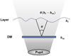 |
Fig. 1 Schematic diagram of single-DM non-conjugate correction. |
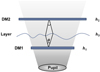 |
Fig. 2 Schematic diagram of multiple-DM non-conjugate correction. |
2.2 Optimization
Based on the derivation in Sect. 2.1, we can conclude that the NCCI quantify the correction capability of the DM in the MCAO system for turbulence layers at different altitudes. Furthermore, by incorporating the turbulence distribution at the telescope site, the NCCI can also evaluate the configuration of the DM. Therefore, for any given turbulence profile  , the overall correction effectiveness of the DM configuration in the MCAO system can be expressed as follows:
 (9)
(9)
The larger the value of NCCItotal, the better the DM in the MCAO system corrects for the given turbulence distribution, indicating a more optimal DM configuration. Thus, the optimization problem for DM configuration can be transformed into finding the optimal value of NCCItotal.
Particle swarm optimization (PSO) is an intelligent optimization algorithm inspired by the foraging behavior of birds (Banks et al. 2007). It simulates a group of birds searching for food within a certain area, where each bird knows the distance to the food. The quickest way to find the food is to search in the vicinity of the bird closest to the food, thereby quickly locating the food. The PSO algorithm follows this rule of a bird flock foraging to solve optimization problems.
The PSO algorithm searches for the optimal solution in the space through group collaboration, making it highly suitable for solving the DM configuration optimization problem. In PSO, each particle represents a potential DM configuration scheme, and particles adjust their positions in the solution space based on their individual experience and the experience of the group. Additionally, the PSO algorithm is suitable for continuous optimization problems and is easy to implement. The steps of the DM configuration optimization algorithm are shown in Algorithm 1.
Each DM conjugate height is considered an element, and multiple elements form a particle. For example, taking a particle with N elements, the i-th particle in the population Xi can be represented as follows:
![Mathematical equation: ${X_i} = \left( {{x_{i1}},{x_{i2}}, \ldots ,{x_{iN}}} \right),{x_{ij}} \in \left[ {0,D{M_{\max }}} \right],j = 1,2, \ldots ,N,$](/articles/aa/full_html/2024/11/aa51919-24/aa51919-24-eq11.png) (10)
(10)
where xij represents the conjugate height of the j-th DM in the i-th particle, ranging from 0 m to the maximum given height.
Require: A population of multiple particles (DM configuration schemes) initialized randomly
Ensure: The optimal DM configuration for the MCAO system under a specific turbulence distribution
1: while the number of iterations is not met do
2: Use Eq. (9) as the fitness function and evaluate the fitness of each particle.
3: Based on the fitness, update the individual best value Pbest and the global best value Gbest.
4: Update the position of the particles according to Eq. (11), obtaining the population xij(t + 1).
5: end while
6: Output Gbest, which is the optimal DM configuration for the MCAO system under the given turbulence distribution.
Before evaluating a particle, we assigned each particle a random initial position, x. Then, we evaluated the particles using a fitness function and updated the particles based on the individual best value, Pbest, and the global best value, Gbest. The fitness function was used to assess the quality of particles, which represents the quality of the DM configuration in this context, and Eq. (9) was used as the fitness function. There are various update rules for the PSO algorithm, and we adopted the standard PSO algorithm update rules:
 (11)
(11)
where w is the inertia weight, which affects the update of particle velocity; c1 and c2 are the learning effects, which control the influence of individual and group experiences on the update; and r1 and r2 are random numbers between 0 and 1, which add randomness to prevent the algorithm getting stuck in local optima. Finally, a conditional check is performed, and if the condition is not met, the process loops until the condition is satisfied. This condition can be the value of NCCItotal or the number of iterations of the algorithm. In this simulation, the number of iterations is chosen.
3 Results and discussions
Simulations were conducted using the Durham Adaptive Optics Simulation Platform (DASP) along with the theoretical model introduced in Sect. 2 for theoretical verification and MCAO performance analysis. DASP is widely used for simulating astronomical and solar AO systems, providing comprehensive analysis of the whole MCAO system performance (Basden et al. 2018). The simulation parameters of the system are shown in Table 1. Additionally, the turbulence models used in this paper are the seven-layer model of Cerro Paranal in Chile (CP7; Ellerbroek & Rigaut 2000) and the seven-layer model of Observatorio del Roque de los Muchachos in the Canary Islands (ORM7; Femenia & Devaney 2003), as illustrated in Fig. 3.
3.1 Simulation tools: Comparison of results
Before conducting the quantification and optimization verification using DASP, we employed two different AO simulation tools – TIPTOP (Quintero Noda et al. 2021), a Fourier-based AO simulation tool, and Object-oriented Matlab Adaptive Optics (OOMAO; Conan & Correia 2014), a Monte Carlo tool – to predict the performance of the MCAO system and ensure the reliability and consistency of the simulation results. We analyzed the MCAO system outlined in Table 1; the turbulence altitudes were set at 0 km, 4 km, 8 km, and 12 km, with corresponding turbulence strength weights of 0.65, 0.25, 0.1, and 0.05, respectively. The conjugate heights of the two DMs were set at 0 km and 8 km. Figure 4 presents a comparison of the performance prediction results from the different simulation tools under these conditions. The results indicate that the outputs from TIPTOP and OOMAO are consistent with DASP, thereby laying a foundation for further quantification and optimization using DASP in subsequent steps.
Simulation parameters of the MCAO system.
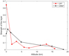 |
Fig. 3 Turbulence profiles used in the simulation. |
3.2 Verification of quantitative methods
This subsection aims to verify the quantification method presented in this paper by comparing the NCCI values obtained from Monte Carlo simulations with those theoretically calculated. We examined the NCCI distribution of MCAO under different DM configurations within the altitude range of 0 to 16 km. Specifically, the DM conjugate heights are (0 km, 6 km), (6 km, 13 km), and (0 km, 13 km). The simulation results are shown in Fig. 5. For the DASP simulation, we calculated the results by placing a single phase screen at different heights hl. Subsequently, we extracted the turbulent phase and the residual phase after MCAO correction for each scientific target direction to compute the structure function. Finally, these values were substituted into Eq. (2) to obtain the NCCI results from the DASP simulation.
Based on MCAO theory, a DM can effectively correct the turbulence layer corresponding to its conjugate height, but the correction effect decreases with increasing distance from the conjugate height. The NCCI reaches near peak values at the DM’s conjugate height and gradually declines to a minimum as the distance increases, which is consistent with theoretical expectations. Furthermore, for this MCAO system, the correction capability of the DM is not confined to a small region a few hundred meters around its conjugate height. In fact, as shown in the figure, a single DM can significantly correct turbulence up to a range of 6 km within a 1-arcmin FOV, with the correction effect extending up to approximately 10 km. Additionally, the closer the spacing between two DMs, the more pronounced the correction effect in the non-conjugate region between them. This indicates that the non-conjugate correction region between DMs in an MCAO system can provide significant turbulence correction, which must be considered when analyzing MCAO system performance.
The NCCI results calculated by DASP align with the overall trend of the NCCI results derived from the method presented in this paper, validating the effectiveness of the theoretical method in quantifying the non-conjugate correction capability of DMs in an MCAO system. However, there is a numerical discrepancy of about 0.05 to 0.1 between the two results, primarily due to various error sources introduced in DASP, such as wavefront sensing errors, wavefront control errors, and noise. Specifically, limitations due to tomography errors, unseen modes, and the overlap of GS footprints in MCAO (Rigaut & Neichel 2018; Femenia & Devaney 2003) often result in the high-altitude DM having less correction capability compared to the low-altitude DM. This situation is also reflected in the figure: the DM at 0 km consistently demonstrates greater correction capability than the DMs at 6 km and 13 km, and the red line representing DASP calculations appears smoother in the vertical profile compared to the blue line. This discrepancy highlights that, in practical MCAO system performance analysis, the correction capability of high-altitude DMs often falls short of theoretical expectations due to wavefront sensing limitations.
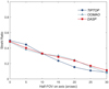 |
Fig. 4 SR as a function of the half-FOV angle with different simulation tools. |
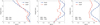 |
Fig. 5 Theoretical calculation of NCCI curves and DASP-calculated NCCI curves. NCCI values are calculated at 1 km intervals across a height range of 0–16 km, resulting in a total of 17 NCCI values. |
3.3 Verification of optimizing methods
In this subsection, the simulation iterations for the PSO algorithm are set to 30, with 20 particles, individual learning effect and group learning effect both set to 1.5, and an inertia weight of 0.8. We first employed an MCAO system with two DMs, with system parameters detailed in Table 1. DM1 was fixed at the pupil plane, and the optimal conjugate height for DM2 was individually optimized.
For the CP7 and ORM7 turbulence models, the PSO optimization results are (0 km, 12.853 km) and (0 km, 11.781 km), respectively. Considering the complexity of designing and implementing an MCAO system, the algorithm-optimized conjugate heights for the high-altitude DM2 are approximately set to 13 km and 12 km. The results of DASP simulations at different conjugate heights for DM2 are shown in Fig. 6. It can be observed that the optimal conjugate heights obtained through Monte Carlo simulations for DM2 remain at 13 km and 12 km. This indicates that the proposed optimization method is effective in optimizing the conjugate heights of a dual-DM MCAO system for common turbulence distributions.
Next, we added an additional DM (DM3) to analyze the optimization results of a three-DM MCAO system; the system parameters are listed in Table 1. For the CP7 and ORM7 models, the PSO optimization results for the three-DM system are (0 km, 3.865 km, 13.281 km) and (0 km, 4.351 km, 12.751 km), respectively. Monte Carlo simulations were conducted to obtain results for different conjugate heights of DM2 and DM3, as shown in Fig. 7. We evaluated 81 combinations of DM2 and DM3 conjugate heights across various height ranges.
Figure 7a shows that for the CP7 model, the optimal conjugate heights obtained from DASP simulations are (0 km, 4 km, 13 km) and (0 km, 4 km, 14 km). Figure 7b shows that for the ORM7 model, the optimal conjugate heights are (0 km, 4 km, 13 km). Compared to the optimized DM configurations obtained using the proposed method, the deviation of the Monte Carlo simulation results for the three-DM MCAO system is less than 1 km. This indicates that the proposed optimization method is accurate and highly practical for MCAO system performance analysis. Additionally, using a laptop with an AMD Ryzen 7 5800H processor, we spent approximately one week simulating 162 different DM combinations using Monte Carlo simulations. In contrast, the proposed optimizing method yielded optimal results in only 5 minutes, significantly reducing the time required for MCAO performance analysis.
Furthermore, for an MCAO system, its performance is highly sensitive to changes in the zenith angle of telescope. This is because the zenith angle directly affects the correction of non-conjugate layers by the MCAO system, resulting in different optimal DM configurations under varying zenith angles. However, the previous simulation results assumed a fixed zenith angle of 0 degrees. Therefore, it is necessary to further explore the optimization of DM configurations under varying zenith angles using the method proposed in this paper.
Using a dual-DM MCAO system as an example, Fig. 8 illustrates the optimized conjugate height of DM2 as the zenith angle increases from 0 to 60 degrees. It can be observed that the conjugate height gradually increases with the zenith angle. When the angle exceeds 40 degrees, the large separation between the DM and the non-conjugate turbulence layers results in more effective correction of lower altitude turbulence compared to higher altitude turbulence. Additionally, the optimization errors between our method and the DASP simulations are mostly within 1 km across the different zenith angles.
It is noteworthy that around a zenith angle of 40 degrees, DASP simulations suggest that placing DM2 at a higher altitude is more beneficial for correcting overall turbulence in the MCAO system, while our optimizing method indicates that positioning DM2 at a lower altitude yields better results. This discrepancy arises primarily due to the introduction of wavefront sensing errors and system errors in DASP. These errors reduce the NCCI of the MCAO system in Monte Carlo simulations compared to the ideal NCCI, indicating that the concentrated correction strategy for low-layer turbulence fails to achieve the theoretical correction level.
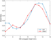 |
Fig. 6 Relationship between the conjugate height of the high-altitude DM and the SR for a dual-DM MCAO system under CP7 and ORM7 turbulence distributions. Results are derived from DASP. |
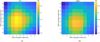 |
Fig. 7 SR distribution for DM2 and DM3 at different conjugate heights in a three-DM MCAO system under CP7 and ORM7 turbulence models. Results are derived from DASP. |
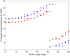 |
Fig. 8 Zenith angle as a function of the conjugate height optimized for DM2. The turbulence models are CP7 (blue) and ORM7 (red), with DM1 fixed at the pupil plane. Circles represent the results from the optimization method proposed in this paper, while triangles represent the DASP simulation results. In the DASP simulations, the conjugate height of DM2 is selected at 1 km intervals. |
3.4 Algorithm performance
In addition to evaluating the accuracy and practicality of the algorithm for optimizing DM configurations within the MCAO system, it is also essential to assess its convergence precision, convergence speed, and robustness. For two turbulence models, CP7 and ORM7, and a three-DM MCAO system, we performed 20 simulations using the PSO algorithm. The results are shown in Figs. 9 and 10.
Regarding the convergence precision of the DM conjugate heights, the error for both DM2 and DM3 is approximately 0.1 km for both the CP7 and ORM7 models. In terms of the convergence precision of NCCItotal, the algorithm consistently converges to the optimal correction value within an average of 30 iterations. This demonstrates that the PSO algorithm provides sufficient convergence precision for optimizing DM configurations.
In Fig. 9a, the convergence error for the DM conjugate heights is higher than in Fig. 9b, which is due to the presence of two peak strengths at high altitudes in the CP7 turbulence distribution, increasing the likelihood of multiple solutions and resulting in a relatively poor convergence precision. The post-convergence NCCItotal for ORM7 is always lower than that for CP7, indicating that the total optimal correction for the MCAO system with a three-DM configuration is consistently less for ORM7 turbulence than for CP7 turbulence. This also explains why the Monte Carlo simulation optimization results for ORM7 are not as good as those for CP7 in Figs. 6 and 7. This phenomenon is also attributed to the presence of two peak strengths at high altitudes in CP7. Although this may increase the convergence accuracy error of the DM conjugate height, the peaks better highlight the height range where layers need correction.
Additionally, Fig. 10 shows that the algorithm converges within 10 iterations, demonstrating very fast convergence speed. Notably, the first iteration significantly optimizes NCCItotal to a relatively high value. The error in the average results of multiple simulations is concentrated in the initial optimization stage, with almost no error during the convergence stage, and the algorithm does not get trapped in local optima. This indicates that the proposed algorithm has a fast convergence speed and sufficient robustness, making it suitable for optimizing DM configurations in MCAO systems.
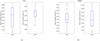 |
Fig. 9 Convergence accuracy of DM2 and DM3 conjugate heights optimized by the PSO algorithm. |
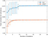 |
Fig. 10 Convergence process of the turbulence total correction NCCItotal in the PSO algorithm. |
4 Conclusions
This study establishes an optimization method for DM configuration in MCAO systems, providing a new theoretical foundation and practical tool for the design and performance optimization of these systems. We conducted theoretical modeling of the non-conjugate correction process of DMs in an MCAO system and analyzed their correction capabilities. Next, we established a DM configuration evaluation criterion, namely NCCI. Using NCCI as the optimal criterion, combined with the PSO algorithm, we searched for the optimal solution within various DM configuration spaces. We utilized the Monte Carlo simulation software DASP for verification, demonstrating the effectiveness of DASP compared to other simulation tools. Furthermore, we compared our proposed theoretical modeling with DASP to verify quantitative and optimizing methods. The DM configurations were also optimized for different zenith angles using our method. Additionally, multiple simulations were conducted to comprehensively evaluate the convergence accuracy, convergence speed, and robustness of the optimization algorithm.
The research results show that the proposed optimization method for DM configuration has two significant advantages in the performance analysis of MCAO systems. First, it quantifies the correction capability of DMs in MCAO, interprets the performance of MCAO systems from the perspective of DM non-conjugate correction, and establishes criteria for DM configuration. Second, based on these quantitative criteria, it establishes an optimization algorithm that provides reasonable DM configuration solutions under any turbulence profile, effectively simplifying the performance analysis process of MCAO systems and improving the efficiency of system optimization. Therefore, this study provides valuable insights for the performance research of MCAO systems and proposes solutions to the problems and limitations in current performance analysis work.
Acknowledgements
The authors would like to thank the reviewers, Xian Ran, Nanfei Yan, Ying Yang, Qianhan Zhou, Junjie Li and Yi Zeng for useful suggestions. This work is supported by the National Natural Science Foundation of China (12103057, 12073031, 12303086), and Youth Innovation Promotion Association, Chinese Academy of Sciences (No. 2021378).
References
- Banks, A., Vincent, J., & Anyakoha, C. 2007, Nat. Comput., 6, 467 [CrossRef] [Google Scholar]
- Basden, A. G., Bharmal, N. A., Jenkins, D., et al. 2018, Softwarex, 7, 63 [NASA ADS] [CrossRef] [Google Scholar]
- Beckers, J. M. 1989, in Active Telescope Systems, 1114 (SPIE), 215 [NASA ADS] [CrossRef] [Google Scholar]
- Beckers, J. M. 2000, SPIE, 4007, 1056 [NASA ADS] [Google Scholar]
- Boccas, M., Rigaut, F., Gratadour, D., et al. 2008, in Adaptive Optics Systems, 7015 (SPIE), 221 [Google Scholar]
- Ciliegi, P., Agapito, G., Aliverti, M., et al. 2024, in Adaptive Optics Systems IX, 13097, SPIE, 1309722 [NASA ADS] [Google Scholar]
- Ciliegi, P., Diolaiti, E., Abicca, R., et al. 2018, in Proceedings of SPIE, 10703, Conference on Adaptive Optics Systems VI [Google Scholar]
- Conan, R., & Correia, C. 2014, in Adaptive optics systems IV, 9148, SPIE, 2066 [NASA ADS] [Google Scholar]
- Crane, J., Herriot, G., Andersen, D., et al. 2018, in Adaptive Optics Systems VI, 10703, SPIE, 1094 [Google Scholar]
- Diolaiti, E., Ragazzoni, R., & Tordi, M. 2001, A&A, 372, 710 [NASA ADS] [CrossRef] [EDP Sciences] [Google Scholar]
- Ellerbroek, B. L., Adkins, S. M., Andersen, D. R., et al. 2012, in Proceedings of SPIE, 8447, Conference on Adaptive Optics Systems III [Google Scholar]
- Ellerbroek, B. L., & Rigaut, F. J. 2000, SPIE, 4007, 1088 [NASA ADS] [Google Scholar]
- Femenia, B., & Devaney, N. 2003, A&A, 404, 1165 [NASA ADS] [CrossRef] [EDP Sciences] [Google Scholar]
- Fusco, T., Conan, J. M., Michau, V., Mugnier, L. M., & Rousset, G. 1999, Opt. Lett., 24, 1472 [CrossRef] [Google Scholar]
- Fusco, T., Conan, J.-M., Rousset, G., Mugnier, L. M., & Michau, V. 2001, J. Opt. Soc. Am. A, 18, 2527 [NASA ADS] [CrossRef] [Google Scholar]
- Fusco, T., Nicolle, M., Rousset, G., et al. 2005, Comp. Rend. Phys., 6, 1049 [NASA ADS] [CrossRef] [Google Scholar]
- Li, Z., Yang, Y., Zhang, L., Huang, L., & Rao, C. 2024, Opt. Lett., 49, 1624 [CrossRef] [Google Scholar]
- Marchetti, E., Hubin, N., Fedrigo, E., et al. 2003, Astronomical Telescopes and Instrumentation, 4839, MAD: the ESO multiconjugate adaptive optics demonstrator (SPIE) [Google Scholar]
- Marchetti, E., Brast, R., Delabre, B., et al. 2007, The Messenger, 129, 8 [NASA ADS] [Google Scholar]
- Neichel, B., Beltramo-Martin, O., Plantet, C., et al. 2021, in Adaptive Optics Systems VII, 11448, SPIE, 603 [Google Scholar]
- Quintero Noda, C., Schlichenmaier, R., Bellot Rubio, L. R., et al. 2022, A&A, 666, A21 [NASA ADS] [CrossRef] [EDP Sciences] [Google Scholar]
- Ragazzoni, R., Marchetti, E., & Rigaut, F. 1999, A&A, 342, L53 [NASA ADS] [Google Scholar]
- Rao, C., Zhong, L., Guo, Y., et al. 2024, PHOTONIX, 5 [Google Scholar]
- Rigaut, F., McDermid, R., Cresci, G., et al. 2021, The Messenger, 185, 7 [NASA ADS] [Google Scholar]
- Rigaut, F., & Neichel, B. 2018, ARA&A, 56, 277 [NASA ADS] [CrossRef] [Google Scholar]
- Rigaut, F. J., Ellerbroek, B. L., & Flicker, R. 2000, Proc. SPIE, 4007, 1022 [NASA ADS] [CrossRef] [Google Scholar]
- Rigaut, F., McDermid, R., Cresci, G., et al. 2020, in Ground-based and Airborne Instrumentation for Astronomy VIII, 11447, SPIE, 378 [Google Scholar]
- Schmidt, D., Gorceix, N., Goode, P. R., et al. 2017, A&A, 597, L8 [NASA ADS] [CrossRef] [EDP Sciences] [Google Scholar]
- Schmidt, D., Beard, A., Ferayorni, A., et al. 2022, Proc. SPIE, 12185 [Google Scholar]
- Tokovinin, A., Le Louarn, M., & Sarazin, M. 2000, J. Opt. Soc. Am., 17, 1819 [NASA ADS] [CrossRef] [Google Scholar]
- Zhang, L., Bao, H., Rao, X., et al. 2023, Sci. China, 66 [Google Scholar]
- Zhang, L., Rao, X., Bao, H., et al. 2024, Astron. Tech. Instrum., 1, 95 [NASA ADS] [Google Scholar]
All Tables
All Figures
|
Fig. 1 Schematic diagram of single-DM non-conjugate correction. |
| In the text | |
|
Fig. 2 Schematic diagram of multiple-DM non-conjugate correction. |
| In the text | |
|
Fig. 3 Turbulence profiles used in the simulation. |
| In the text | |
|
Fig. 4 SR as a function of the half-FOV angle with different simulation tools. |
| In the text | |
|
Fig. 5 Theoretical calculation of NCCI curves and DASP-calculated NCCI curves. NCCI values are calculated at 1 km intervals across a height range of 0–16 km, resulting in a total of 17 NCCI values. |
| In the text | |
|
Fig. 6 Relationship between the conjugate height of the high-altitude DM and the SR for a dual-DM MCAO system under CP7 and ORM7 turbulence distributions. Results are derived from DASP. |
| In the text | |
|
Fig. 7 SR distribution for DM2 and DM3 at different conjugate heights in a three-DM MCAO system under CP7 and ORM7 turbulence models. Results are derived from DASP. |
| In the text | |
|
Fig. 8 Zenith angle as a function of the conjugate height optimized for DM2. The turbulence models are CP7 (blue) and ORM7 (red), with DM1 fixed at the pupil plane. Circles represent the results from the optimization method proposed in this paper, while triangles represent the DASP simulation results. In the DASP simulations, the conjugate height of DM2 is selected at 1 km intervals. |
| In the text | |
|
Fig. 9 Convergence accuracy of DM2 and DM3 conjugate heights optimized by the PSO algorithm. |
| In the text | |
|
Fig. 10 Convergence process of the turbulence total correction NCCItotal in the PSO algorithm. |
| In the text | |
Current usage metrics show cumulative count of Article Views (full-text article views including HTML views, PDF and ePub downloads, according to the available data) and Abstracts Views on Vision4Press platform.
Data correspond to usage on the plateform after 2015. The current usage metrics is available 48-96 hours after online publication and is updated daily on week days.
Initial download of the metrics may take a while.