| Issue |
A&A
Volume 684, April 2024
|
|
|---|---|---|
| Article Number | A183 | |
| Number of page(s) | 11 | |
| Section | Astronomical instrumentation | |
| DOI | https://doi.org/10.1051/0004-6361/202348346 | |
| Published online | 22 April 2024 | |
SMART: Special-shaped Micro-lens Aimer for Real-time Targeting of multi-object telescopes
1
Key Laboratory of In-Fiber Integrated Optics of Ministry of Education, College of Physics and Optoelectronic Engineering, Harbin Engineering University,
Harbin
150001, PR China
e-mail: sunweimin@hrbeu.edu.cn
2
Key Laboratory of Photonic Materials and Devices Physics for Oceanic Applications, Ministry of Industry and Information Technology of China, College of Physics and Optoelectronic Engineering, Harbin Engineering University,
Harbin
150001, PR China
3
Qingdao Innovation and Development Center of Harbin Engineering University,
Qingdao
266000, PR China
4
Yantai Research Institute and Graduate School of Harbin Engineering University,
Yantai
264000, PR China
5
State Key Laboratory of Aerodynamics, China Aerodynamics Research and Development Center,
Mianyang
621000, PR China
Received:
22
October
2023
Accepted:
8
February
2024
In the process of acquiring astronomical spectral data, the alignment accuracy between the fiber core in the focal plane and the image of the target star is crucial for multi-target telescopes. This work presents a Special-shaped Micro-lens Aimer for Real-time Targeting (SMART), which combines a special-shaped microlens and a fiber bundle to carry out online alignments and improve the injection efficiency of the fiber. The special-shaped microlens consists of a central plate and six side microlenses. The central plate transfers the signal to the science fiber without focal ratio degradation. The side microlenses focus the leakage light to the feedback fibers and return a misalignment signal. The experiment in the laboratory indicates that the SMART-T system can visually demonstrate the recognition of offsets. The SMART-P system is able to realize the alignment for a variety of seeing cases. Under the condition that the diameter of turbulent star image is 0.2 mm, the corrected injection efficiency is improved to 99.7% of the best injection efficiency of the science fiber. The re-centering accuracy is 0.01 mm.
Key words: instrumentation: spectrographs / techniques: miscellaneous / techniques: spectroscopic / telescopes
© The Authors 2024
 Open Access article, published by EDP Sciences, under the terms of the Creative Commons Attribution License (https://creativecommons.org/licenses/by/4.0), which permits unrestricted use, distribution, and reproduction in any medium, provided the original work is properly cited.
This article is published in open access under the Subscribe to Open model. Subscribe to A&A to support open access publication.
1 Introduction
In recent decades, large-scale spectroscopic surveys have enormously improved our understanding of the content and evolution of the Universe (da Cunha et al. 2017). One key tool is the multi-fiber telescope, used to observe thousands of targets at the same time (Zhang et al. 2018). The optical fiber increases the spectral acquisition rate and makes large-scale spectroscopic surveys possible thanks to the long-distance transmission property and flexible characteristics (Smith et al. 2004). With the increasing complexity and scale of astronomical phenomena, astronomical instruments are required to sample larger and deeper (Morales et al. 2012). The integrated number of the fiber on the focal plane of the multi-object telescope has been increasing, from 400 for the Anglo Australian Telescope (AAT Smith & Lankshear 1998) to 4000 for the Large Sky Area Multi-Object Fiber Spectroscopic Telescope (LAMOST Cui et al. 2012), and 5000 of Mayall Telescope (Edelstein et al. 2018).
Fibers are mounted on the focal plane by the well-known fiber positioner units (FPU), such as a labor-intensive plug-plate (Wan et al. 2006; Smee et al. 2013; Owen et al. 1994), pick-and-place with a replaceable focal plane (Barden 2004; Lewis et al. 2002), parallel-operated method including double-revolving (Su & Cui 2003; Hu et al. 2018), tilting spine (de Jong et al. 2012), and starbug (Staszak et al. 2016; Gilbert et al. 2012). The misalignment between the star image and the fiber core leads to energy loss and focal ratio degradation (Sun et al. 2016) in the medium- and low-resolution spectrometer. And it also results in the reduction of the spectrum resolution due to the centroid shift of the spot energy at the output of the fiber (Ishizuka et al. 2016) in the high-resolution spectrometer. Hence, fiber position detection is crucial to FPU.
LAMOST is an innovative reflecting Schmidt telescope, with one of its key technologies being the original double-revolving fiber positioning technology. It uses an open-loop system to control the FPU in the early stage (Zhou et al. 2021a). Prior to observation, all FPUs have to return to their initial positions before new configurations can be performed. Later, the back-illumination method was proposed, whereby light enters fibers from the spectrometer end and the other end of the fibers is imaged via a vision system. However, the illumination device brings mechanical instability in the spectrograph and reduces the efficiency of astronomical observations (Zhou et al. 2021b). As a result, the front-illuminated method has been presented, whereby the fiber end is photographed and characteristic points are extracted to analyze the fiber position. Compared with the back-illuminated method, this approach reduces the device complexity and improves the efficiency of the observation. Nonetheless, during long-term observations, the fiber position may change due to the mechanical jitter of the telescope, the collision between the FPUs, or the rotation of the earth. Therefore, real-time monitoring of the relative position between the star image and the fiber core is significant in improving the signal-to-noise ratio (S/N) of spectral observations. To address this issue, Yang et al. (2018) proposed a five-core fiber for LAMOST, which consists of a science fiber core and four feedback fiber cores. However, when the star image deviates from the science fiber core and falls in the gap between the science fiber core and the feedback fiber cores, the offset cannot be detected.
In this paper, we propose a Special-shaped Microlens Aimer for Real-time Targeting (SMART) installed in front of the fiber of a telescope. SMART consists of a special-shaped microlens and a fiber bundle, which is designed on the basis of optical simulations. Through the signal of the feedback fibers, SMART can correct the offset of the science fiber core relative to the star image during astronomical observation and realize the realtime monitoring without blind area. The SMART is a potential candidate of auto-allignment devices in multi-fiber telescopes.
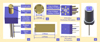 |
Fig. 1 Schematic diagram of SMART, (a) Structure of SMART, (b) Front surface of SMA. (c) Cross-section of SMA. (d) FPM. (e) Detecting FPM. (f) Design of SMART. |
2 Design for SMART
We present SMART to achieve real-time calibration of fiber position to improve the injection efficiency of the science fiber. As shown in Fig. 1a, SMART consists of a special-shaped microlens array (SMA) and a fiber bundle. The front surface and cross-section of SMA are shown in Figs, 1b and c. It includes a round central plate in the middle and six fan-shaped planoconvex lenses around it. The central plate ensures that the beam entering the science fiber without any change in terms of the focal ratio. The fan-shaped lens achieves a continuous detection space between the science fiber core and the feedback fiber core. The fiber bundle consists of one science fiber and six feedback fibers. The science fiber is used to transmit the starlight from the focal plane to the spectrometer. The feedback fibers are applied to recognize the offset between the science fiber core and the star image. One end of the fiber bundle is fixed in a fiber positioning microplate (FPM Fig. 1d) to connect with SMA. The other end of the fiber bundle was tested in the experiment using two methods. In one method, the other end of the fiber bundle is inserted in the detecting FPM (Fig. 1e). A CCD is used to capture the near field of fibers when detecting FPM to visually demonstrate the alignment performance of SMART during laboratory testing. In the other method, light from the science fiber is transported to optical power meter. The star light strayed from the central plate is coupled to the feedback fiber through the fan-shaped lens and transmitted to the photo-detector to obtain the offset signal. Figure 1f shows the design of SMART.
An ideal point source is considered as the star image for the optical design of SMART. To facilitate the manufacture, the thickness of the central plate is designed to be 2.500 mm and the plano-convex lens is thicker than the central plate. The optical path design of the central plate is shown in Fig. 2a. When star light enters the central plate, the star image focuses on the science fiber core.
The diameter, D0, of the central plate is determined by the core diameter d0 of the science fiber and the spot radius, r0, on SMA surface. The relationship between D0, d0, and r0 is expressed as Eq. (1):
 (1)
(1)
The spot radius, r0, on the SMA surface is related to the tilt angle, θ, of the incident light, thickness, H, and refractive index, n′, of SMA:
 (2)
(2)
We consider that the output focal ratio of LAMOST is F/5:
 (3)
(3)
where d0 is 0.320 mm (LAMOST fiber core diameter), thickness Η is 2.500 mm, and n′ of SMA is 1.523, the diameter of the central plate was determined to be 0.647 mm.
Six plano-convex lenses are used in SMA to achieve a compact structure and the width of each plano-convex lens is 0.200 mm. The optical path for radius design of the plano-convex lens is shown in Fig. 2b. Mirror b (Mb) of the LAMOST system is chosen to be the aperture stop in the optical system. Mb is also the enter pupil of the optical system. The imaging of Mb by the fan-shaped lens is the exit pupil of the system, which is the export of the output beam. Therefore, the position of the exit pupil is designed on the back surface of SMA, which is also the front surface of the fiber. In simulation, according to the known thickness and the refractive index of the lens, and the distance between the front surface of lens and Mb, the initial curvature radius, R, of the fan-shaped lens can be obtained as 0.973 mm. Nevertheless, the curvature radius, R, of the lens needs to be designed comprehensively with the diameter and position of the feedback fiber core. The curvature radius, R, of the plano-convex lens is finally determined to be 0.960 mm and the core diameter of the feedback fiber is 0.105 mm. The design parameters of SMART are shown in Table 1.
The light of each target star is concentrated on the core of the corresponding fiber through the optical system of the telescope. When a fiber in the focal plate of a telescope is replaced with SMART, the starlight first passes through SMA and then enters the fiber. In SMART, when there is no offset between the science fiber and the starlight, the star light pass through the central plate, as shown in Fig. 2c. The star beam enters the core of the science fiber without changing focal ratio. When there is an offset between the science fiber and the star image gathered by the telescope, as shown in Fig. 2d, the light overflowing from the central plate will enter the plano-convex lens. Then the lens deflects the light into the core of the feedback fiber. Because of the design of the plano-convex lens, there is no blind area at all directions. In another words, as soon as the star light offsets the central plate, energy will be collected in the feedback fibers. Comparing the energy collected in six feedback fibers, we can estimate the direction and distance of the offset between the science fiber and the star image.
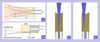 |
Fig. 2 SMA design and function diagram, (a) Central plate design light path diagram, (b) Plano-convex lens, (c) Light path with no offset between the science fiber and the star image, (d) Light path with an offset between the science fiber and the star image. |
Design parameters of SMART.
3 Simulation of SMART performance based on the Fresnel diffraction theory
3.1 Theoretical model
According to the parameter of LAMOST system, the telescope is simplified to a lens with the same output focal ratio of F/5 as shown in Fig. 3a. The offset starlight passes through the simplified telescope system. The star light on the front surface of the central plate and the fan-shaped lens is concentrated on the rear surface of the central plate and the lens, separately. To explore the energy distribution of the star image on the rear surface of SMA when the star beam incident at different positions on the front surface of SMA, we established a simulation model by using Fresnel diffraction theory. Fresnel diffraction integral is shown in Eq. (4):
 (4)
(4)
where the diffraction aperture is in the plane (ξ, η), and the observation plane is in the plane (x, y). The two planes are parallel with the normal distance of z. Then, k is the wave number and λ is the wavelength in vacuum. As shown in Fig. 3a, when the parallel starlight enters the simplified telescope system, the light field on its front and back surfaces are U0(ξ, η) and U1(ξ, η). The light field propagating to the central plate and the lens on the front surface of SMA are U2p(u, v) and U21(u,v), respectively. The light field converging on the back surface of the central plate is U3p(x, y). The light field deflected to the back surface of the lens is U3(x, y).
Figure 3b shows the front surface of SMA. The angle of the offset direction is a, and the displacement is l. Line AB is the threshold width of the star spot entering the front surface of SMART, which is 0.324 mm. It is worth noting that when the spot diameter is less than the threshold width AB, at most two adjacent feedback fibers will collect light energy. Figure 3c shows the star image distribution on the rear surface of SMART when the star light is offset. The image is shifted out of the science fiber core, and the star energy entering the fan-shaped lens focuses on feedback fibers 1 and 2.
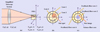 |
Fig. 3 Simulation model of the offset between the star image and SMA. (a) Simplified telescope optical system, (b) Star light offset on the front surface of SMA. (c) Star image offset on the rear surface of SMA. |
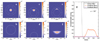 |
Fig. 4 Simulation results along α = 90° without turbulence, (a, b) The spot pattern of the front and rear surfaces of the central plate when there is no relative offset between SMA and the star image, (c, d) Spot pattern of the front and rear surfaces of the central plate when the displacement is 0.27 mm. (e, f) Spot pattern of the front and rear surfaces of lens 1 when the displacement is 0.27 mm. (g) Energy of fibers at different displacement distances when α = 90°. |
3.2 Simulation without atmospheric turbulence
The star spot diameter on the front surface of SMART is 0.327 mm, which is less than the threshold width AB. Lenses 1 and 2 are chosen to be studied. Three offset angles α are selected to be 90°, 72°, and 60°.
Figures 4–6 show the simulation results when α are 90°, 72°, and 60° and the displacement is 0.27 mm. The front surface of SMART is shown in (a), (c), and (e) of Figs. 4, 5, and 6, where the round and fan-shaped areas stand for the central plate and the fan-shaped lenses of SMART. The rear surface of SMART is shown in (b), (d), and (f) of Figs. 4, 5, and 6, where big circles and small circles represent the science fiber core and the feedback fiber core. The relationship between the displacement and the energy collected by the fibers is described in (g) of Figs. 4, 5, and 6. Without regard to the influence of numerical aperture (N.A.) and the transmission loss of the fibers, we consider the integral of energy in the circle to represent the energy collected in the fiber.
In Fig. 4, the star light moves along α = 90°. The offset star light only enters the lens 1. Only feedback fiber 1 gains energy. Since the core diameter of the science fiber is 0.32 mm, the star light is offset from the central plate to the fan-shaped lens when the displacement is 0.16 mm. Therefore, in Fig. 4d, the star light entering the center plate is focused outside the science fiber core. In Fig. 4f, it shows that the star light falling on lens 1 produces an irregular light field distribution. Part of the light field is collected by feedback fiber 1. Under different displacement, the light field has different shapes and positions, which leads to energy changes in feedback fiber 1. Although not all the light enters feedback fibers, the energy collected by it is sufficient to reflect the variation of the displacement within a certain range. In Fig. 4g, the energy collected in the science fiber remains the same before the displacement is 0.16 mm. After that, it quickly drops to zero. The energy change in feedback fiber 1 goes through the stages of non-response, energy rise, flat, and decline, corresponding to the whole process of star light moving from the center of the central plate to the edge of the plate, and then into the fan-shaped lens, until away from the lens.
In Figs. 5 and 6, the star light enters lenses 1 and 2 at the same time, and both feedback fibers 1 and 2 gain energy. When the star light moves along α = 72°, it can be seen from Fig. 5g that most energy of the star light is collected by feedback fiber 1 and a small part is gathered by feedback fiber 2. This can also be reflected from the light field distribution in Figs. 5d and f. When α = 60° (seen in Fig. 6), the star image on the front surface of SMA is bisected by the microlens corresponding to the feedback fiber 1 and 2, resulting in an equal output energy (seen in Fig. 6g).
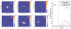 |
Fig. 5 Simulation results along α = 72° without turbulence, (a, b) Spot pattern of the front and rear surfaces of the central plate when the displacement is 0.27 mm. (c–f) Spot pattern of the front and rear surfaces of lens 1 and lens 2 when the displacement is 0.27 mm. (g) Energy of fibers at different displacement when α = 72°. |
 |
Fig. 6 Simulation results along α = 60° without turbulence, (a, b) Spot pattern of the front and rear surfaces of the central plate when the displacement is 0.27 mm. (c–f) Spot pattern of the front and rear surfaces of lens 1 and lens 2 when the displacement is 0.27 mm. (g) Energy of fibers at different displacement when α = 60°. |
3.3 Simulation with atmospheric turbulence
In astronomical observation, due to atmospheric turbulence, the imaging quality demand of LAMOST is 80% light energy within 2 arcsec (Bai & Yuan 2010), which means that the diameter of the star image is 0.2 mm. During the simulation with atmospheric turbulence, the position of the star image on the rear surface of SMART is influenced by the inclination angle of the parallel light incident into the simplified telescope. Figures 7–9 show the simulation results with atmospheric turbulence when α are 90°, 72°, and 60° and the displacement is 0.27 mm. A total of 182 parallel light of different incident angles were simulated as the turbulence image spots on the back surface of SMA, as shown in Fig. 7b. The sum of the energy of all incident light is the same as the energy of one incident light beam without turbulence.
When the turbulent spot in the focal plane is 0.2 mm, the diameter of the star spot on the front side of the central plate is 0.527 mm, which is greater than the threshold width AB of the fan-shaped lens. When α = 90°, up to three feedback fibers will get the signal. However, as can be seen from Fig. 7g, almost no signals are collected in feedback fibers 2 and 6, so the images of lens 2 or 6 are not given. In the other two offset directions, the star light only enters two lenses. Compared with the simulation results without turbulence, the diameter of the star spot on the front surface of SMA increases in the presence of turbulence, but the maximum value of the spot energy decreases.
This is because turbulence causes the spot expanded and the energy to become less concentrated. The light field distribution varies greatly on the rear surface of SMA. When the l is 0 mm, the star image with a diameter of 0.2 mm on the focal plane is simulated as shown in Fig. 7b, which is composed of single image points with Gaussian distribution. When the l is not 0 mm, the light field distribution on the back surface of lenses 1 and 2 is expanded, the shape is changed, and the energy is obviously decreased.
The energy distribution of the spot on the front face of SMA is Gaussian. The energy of the science fiber decreases at the displacement of 0.04 mm. In the feedback fiber, the signal will be obtained earlier than that without turbulence. Moreover, the displacement of peak energy in the feedback fiber increases.
According to the simulation results in this section, it can be concluded that the relative offset state between the star image and the science fiber core can be judged by the signal in the feedback fiber of SMART with and without turbulence. The correction of SMART position can be guided to improve the injection efficiency of science fiber.
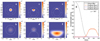 |
Fig. 7 Simulation results along α = 90° with turbulence, (a, b) Spot pattern of the front and rear surfaces of the central plate when there is no relative offset between SMA and the star image, (c, d) Spot pattern of the front and rear surfaces of the central plate when the displacement is 0.27 mm. (e, f) Spot pattern of the front and rear surfaces of lens 1 when the displacement distance is 0.27 mm. (g) Energy of fibers at different displacement when α = 90°. |
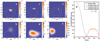 |
Fig. 8 Simulation results along α = 72° with turbulence, (a, b) Spot pattern of the front and rear surfaces of the central plate when the displacement is 0.27 mm. (c-f) Spot pattern of the front and rear surfaces of lens 1 and lens 2 when the displacement is 0.27 mm. (g) Energy of fibers at different displacement when α = 72°. |
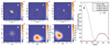 |
Fig. 9 Simulation results along α = 60° with turbulence, (a, b) Spot pattern of the front and rear surfaces of the central plate when the displacement is 0.27 mm. (c–f) Spot pattern of the front and rear surfaces of lens 1 and lens 2 when the displacement is 0.27 mm. (g) Energy of fibers at different displacement when α = 60°. |
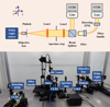 |
Fig. 10 Schematic diagram of the experimental setup for SMART-T. |
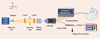 |
Fig. 11 Stucture diagram of SMART-R |
4 Experiment
4.1 Optical setup
In the experiment, two SMART systems were tested. One is shown in Fig. 10, which includes the SMA, fiber bundle, and detecting FPM. It is called testing SMART (SMART-T) to visually show the performance of SMART. The other is shown in Fig. 11, which consists of an optical power meter and a six-channel photo-detector. It is named prototype SMART (SMART-P), to highlight the detection of the energy of the fibers precisely.
The optical setup for testing the performance of SMART-T is shown in Fig. 10. The white-light source was converged by an objective lens with a magnification of 40x and a numerical aperture of 0.4. A pinhole is placed in the object plane of the collimator. Then, the light was collimated by lens 1 with a focal length of f = 75 mm. To simulate the F/5 focal ratio of the LAMOST output beam, an aperture stop of a diameter of 15 mm and lens 2 with the same focal length as len 1 were used. A lensed camera labeled CCD1 with a resolution of 3296 × 2472 and a pixel pitch of 5.5 μm (Prosilica GT3300, Allied Vision Technologies Co., Ltd.) was applied to capture the spot energy on the surface of the detecting FPM. Another CCD2 with a resolution of 5496 × 3672 and a pixel pitch of 2.4 μm (MER2-2000-19U3M, Daheng Optics Co., Ltd.) was used to capture the image of the front surface of SMA.
Then, to accurately measure the intensity of the signals inside the science fiber and the feedback fiber, we replaced SMART-T with SMART-P. As shown in Fig. 11, an optical power meter (Thorlabs Co., Ltd.) was used to measure the light energy collected in the science fiber core. A six-channel photo-detector (CH253, HAMAMATSU Co., Ltd.) was applied to detect the signals from six feedback fibers whose six channels have been calibrated.
4.2 SMART-T measurement
Firstly, the optics setup had to be aligned. Next, to simulate the atmospheric turbulence, a pinhole with a diameter of 0.2 mm was used, which was then adjusted with a shearing interferometer (SI500, Thorlabs Co., Ltd.) to generate a collimated light. CCD2 was employed to observe the position of the incident beam on the front surface of SMA. Then, we moved the position of SMART-T so that the star light is centered on its front surface. This position is marked as the initial position and remains constant for each test. Finally, SMART-T is moved along α = 90°, 72°, and 60°, with each step of 0.01 mm and a total of 0.5 mm. CCD1 was used to obtain the gray value of fibers in detecting FPM at different offset directions and distances. The sum of the gray value in the core region of each fiber is considered to be the energy received by it.
4.3 SMART-P test under various seeing cases
Due to the variable seeing cases that existed in astronomical observation, we selected four different size of pinholes to represent four seeing cases, whose diameters are 0.05 mm, 0.1 mm, 0.15 mm, and 0.2 mm, respectively. After replacing the pinhole, the energy of the white light source is adjusted to ensure that all the energy entering the SMART is the same. Under each seeing case, SMART-P is moved along α = 90°, 72°, and 60°, with each step of 0.01 mm and a total of 0.5 mm. The energy intensity of the signal in the science fiber and the feedback fiber was recorded when moving to each position.
4.4 SMART-P test of re-centering accuracy
The position correction ability of SMART-P was tested with a pinhole diameter of 0.2 mm. Firstly, the noise of the six-channel photo-detector was measured without a light source. Then, under white light, the position of SMART-P was adjusted according to the optical power meter to achieve the best injection state of the science fiber. The energy entering into SMART-P was also detected to obtain the injection efficiency in the best injection state. The energy in the six feedback fibers measured by the six-channel photo-detector is defined as the benchmark signal of each of the six fibers. Next, a known random offset was injected into SMART-P. The intensity in the science fiber was measured to acquire the injection efficiency after the offset. Finally, the relative position between SMART-P and the star image was adjusted according to the signal in the feedback fiber. The injection efficiency of science fiber was detected again. Finally, the re-centering performance under 20 random offsets was tested. All the experimenter conditions are given in Table 2.
Experiment conditions.
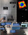 |
Fig. 12 Whole structure of the SMART system. (a) Photo of the SMART-T system. (b) Interferogram of the front surface of SMA. (c) Detecting FPM illuminated by parallel light from SMA. (d) Photo of the SMART-P system. |
5 Results and discussion
5.1 Structure of the SMART system
The photo of the SMART-T system is shown in Fig. 12a. There are three parts in the SMART-T system: the input end, output end, and fiber bundle. The input end including SMA and the FPM is used to receive the incident beam. Figure 12b shows the interferogram of SMA fabricated by injection molding method1. Therefore, a height difference between the SMART central plate and the microlens is designed to facilitate the making of molds. The shape of SMART was changed to a square for easy demolding and it did not change the performance of design. The seven fibers in the fiber bundle were inserted and bonded in the detecting FPM to be the output end. Figure 12c shows the detecting FPM illuminated by parallel light from SMA. Figure 12d shows the SMART-P system, which consists of the input end, optical power meter, and six-channel photo-detector.
5.2 Performance of the SMART-T system
To simulate the atmospheric turbulence, we selected a pinhole with a diameter of 0.2 mm to be the object. Since an optical 4F system is used in the optical path, the diameter of the spot on the rear surface of the SMART is approximately considered to be 0.2 mm. To show the results of the SMART system intuitively, we exhibited the grayscale map of the fibers in the detecting FPM photographed by CCD1 with the SMART system offset along different directions and different displacement relative to the light source. In Figs. 13a-c are near field of fibers with offset directions along α = 90°, 72°, and 60°, respectively. Each image shows seven offset position states, from 0.12 mm to 0.36 mm, with a step of 0.04 mm.
When the spot on the front surface of SMART is offset along α = 90°, it enters three lenses theoretically. While, in Fig. 13a, only feedback fiber 1 collects light energy. This is because the intensity of the light energy collected in the feedback fibers 2 and 6 is too small to be observed. As the displacement increases, the light energy intensity in the science fiber decreases, and the light energy intensity in the feedback fiber 1 increases. In Fig. 13b, when the spot is offset along the direction of α = 72°, energy inequality in feedback fibers 1 and 2 can be observed. In Fig. 13c, when the α = 60°, half of the energy of the spot enters lens 1 and the other half enters lens 2. The energy collected in feedback fibers 1 and 2 is nearly equal.
5.3 Performance of the SMART-P system under various seeing cases
The relationship between the displacement and the normalized energy collected in the feedback fibers, along α = 90°, 72°, and 60° is tested under various seeing cases, as shown in Fig. 14. The x-coordinate represents the displacement l, ranging from 0 to 0.5 mm, with a marker of 0.01 mm intervals. The y-coordinate on the left and right represent the normalized energy of the science fiber and the feedback fiber, respectively.
The trend of energy change in the science fiber is analyzed first, which is consistent with simulation results. As in Fig. 14, the energy decreases slowly at first. And when the pinhole becomes larger, the gentle descent region becomes smaller. This is caused by the increasing diameter and decreasing concentration of energy distribution of the boundary-less star image (as mentioned in Sect. 3.2). In the experimental, the energy collected in the science fiber decreases when the displacement is smaller, due to the coupling energy loss of the fiber. Compared with the simulation results, the rapid drop region is caused by a large amount of energy of the star image shifting out of the science fiber core. When the seeing is worse, the energy of the star image escapes more easily from the science fiber core, so the rapid descent region is longer. When the spot is away from the science fiber core, almost no energy exists in the science fiber.
The energy variation trend of the feedback fiber also agree with the simulation result. When α = 90°, only feedback fiber 1 obtains the signal under different seeing conditions. Feedback fiber 1 first has an irresponsive region, which means that most of the energy of the star image does not enter the fan-shaped lens. As the diameter of the turbulent star image increases, the irresponsive region becomes smaller. Then, the energy in feedback fiber 1 rises rapidly with the increase of the displacement, which represents that the main energy of the star image enters the microlens. Finally, the energy in feedback fiber 1 is relatively stable because the main energy of the star image does not leave the microlens. This is not consistent with the simulation results, because the turbulence image is slightly larger than 0.2 mm due to the influence of diffraction and aberration.
When α = 72°, the curve of feedback fiber 1 in α = 72° is same as the curve in α = 90°. In feedback fiber 2, as the turbulent spot becomes larger, the peak value of the signal becomes larger. The reason for this is that as the diameter of the turbulent spot became larger, the light field distribution range on the back surface of SMA increases in the offset state and more energy enters the feedback fiber. The displacement of the signal obtained by feedback fiber 2 is greater than that of feedback fiber 1, which is due to less spot energy entering lens 2.
When α = 60°, similarly, as the pinhole increases, the irresponsive zone of the feedback fiber becomes smaller. However, at the same displacement, compared with the energy in the feedback fiber 1 at α = 90°, the energy in the fiber decreases, and the irresponsive zone increases. This is because the two lenses divide the total energy of the star image equally. This also results in an obvious downward trend in the feedback fiber signal when the displacement is large.
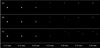 |
Fig. 13 Near field of fibers in the detecting FPM. (a) SMART moves along α = 90°. (b) Along α = 72°. (c) Along α = 60°. |
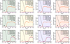 |
Fig. 14 Energy of fibers at different displacement under various seeing cases, (a–c) Diameter of pinhole is 0.05 mm. (d–f) Diameter of pinhole is 0.10 mm. (g–i) Diameter of pinhole is 0.15 mm. (j–1) Diameter of pinhole is 0.20 mm. |
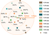 |
Fig. 15 Position of 20 known random offsets and the science fiber injection efficiency at this position. |
5.4 Re-centering performance of the SMART-P system
To test the offset correction performance of the SMART-P system between the science fiber and the star image during astronomical observation, we injected 20 known random offsets with a pinhole diameter of 0.2 mm for testing.
First, the mean value of the best injection efficiency of the science fiber is 85.0%. The loss of injection efficiency may be due to the lack of film-coating on the SMART front surface and the coupling loss. In the best injection state, the dark current noise of the six-channel photodetector is 0.004 mV, 0.002 mV, 0.004 mV, 0.002 mV, 0.003 mV, and 0.003 mV, respectively. When the white light source is turned on, the signals of the six feedback become 0.145 mV, 0.092 mV, 0.116 mV, 0.105 mV, 0.115 mV, and 0.160 mV; these are used as the benchmark signal. The signal in the feedback fiber becomes larger because the star spot on the front surface of the SMART-P is boundless and a small amount of energy falls on the front surface of fan-shaped lens. It may also because the surface scattering and the reflection between the upper and lower surfaces of SMA. Then the position of SMART-P is adjusted to offset the center of the star image. The position of the 20 offsets is shown in Fig. 15, and the injection efficiency of the science fiber at each position is also shown. After that, the state of SMART-P was corrected according to the six feedback signals.
During the re-centered process, the visibility of the signal intensities of the two fibers spaced 180° apart is used as the calibration criterion. The visibility is the ratio of the difference to the sum between signal intensities of two feedback fibers placed at 180° and it is defined as in Eqs. (5)–(7):
 (5)
(5)
 (6)
(6)
 (7)
(7)
where I1 to I6 represent the signal obtained by feedback fiber 1 to 6.
The visibility of the benchmark signals is Vb1 = 0.160, Vb2 = −0.111, and Vb3 = −0.159. The differences of the visibility ΔV1, ΔV2, and ΔV3 between the benchmark signal and the signal after 20 re-centering are given as shown in Fig. 16. It is defined that the re-centering process has been completed when the visibility difference is less than 0.150.
Finally, the injection efficiency of the science fiber after 20 offset corrections is shown in Fig. 17. The average injection efficiency is 84.8%, which is 99.7% of the best injection efficiency. Compared with the offset and energy curve tested under the pinhole with a diameter of 0.2 mm in Sect. 5.3, the re-centering accuracy of the SMART-P system can reach 0.01 mm.
The test results are not quite the same as the theoretical design. The test results show that, when the displacement is 0.01 mm, the SMART-P system can recognize it. SMART is designed from geometrical optics, the feedback fiber will collect signals if the star image is offset from the science fiber core. However, there is no clear boundary of the star image in practice. Even there is no offset between the center of the star image and the center of the science fiber, the signal will also be obtained in the feedback fiber due to the small energy at the edge of the spot. In addition, there may be scattering in SMA (the material is not ideal uniform) and the six-channel photo-detector used has low noise and high accuracy. All of these are the reasons why the signal is collected in the feedback fiber but the star image has not been shifted out of the science fiber core. Therefore, the measurement accuracy of SMART-P is closely related to the energy distribution of the light source and the detection accuracy of the photo-detector of feedback fibers.
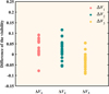 |
Fig. 16 Difference of the visibility. |
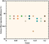 |
Fig. 17 Science fiber injection efficiency after 20 known random offsets were corrected. |
6 Conclusion
Based on a special-shaped microlens and a fiber bundle, this paper presents the SMART system, which can estimate the relative position of the target star image and the science fiber core in real-time. According to the observation conditions of LAMOST, we designed the surface shape and size of the special-shaped microlens and selected the parameters and position of the feedback fibers. Then, we used the Fresnel diffraction propagation model to simulate the relationship between the energy collected by the feedback fiber and the displacement under different offset directions with and without atmosphere turbulence. Eventually, the SMART-T system is used to visually show the recognition of offsets. The SMART-P system is applied to collected the data. The performance of the SMART-P system was tested under various seeing cases in the lab. The test results show that it can realize the alignment between star image and science fiber core under different seeing cases. The re-centering accuracy is tested when the diameter of the turbulent star image is 0.2 mm. The corrected injection efficiency is 99.7% of the best injection efficiency of the science fiber. The re-centering accuracy of the SMART-P system can reach 0.01 mm. The next generation of SMART will be fabricated using high-precision technologies such as laser direct writing. The front surface of SMART will be coated to improve the injection efficiency of science fiber.
Acknowledgements
This work was supported by the Joint Research Fund in Astronomy under cooperative agreement between the National Natural Science Foundation of China (NSFC) and Chinese Academy of Sciences (CAS) under U2031132; the Fundamental Research Funds for the Central Universities to the Harbin Engineering University under 3072022QBZ2501.
References
- Bai, H., & Yuan, X. Y. 2010, Adaptive Optics Systems II, 7736 [Google Scholar]
- Barden, S. C. 2004, SPIE Conf. Ser., 5492, 75 [NASA ADS] [Google Scholar]
- Cui, X. Q., Zhao, Y. H., Chu, Y. Q., et al. 2012, Res. Astron. Astrophys., 12, 1197 [Google Scholar]
- da Cunha, E., Hopkins, A. M., Colless, M., et al. 2017, PASA, 34, e047 [NASA ADS] [CrossRef] [Google Scholar]
- de Jong, R. S., Chiappini, C., & Schnurr, O. 2012, Assembling the Puzzle of the Milky Way, EPJ Web Conf., 19, 09004 [NASA ADS] [CrossRef] [EDP Sciences] [Google Scholar]
- Edelstein, J., Jelinsky, P., Levi, M., et al. 2018, Proc. SPIE, 10702, 107027G [NASA ADS] [Google Scholar]
- Gilbert, J., Goodwin, M., Heijmans, J., et al. 2012, Proc. SPIE, 8450, 84501A [NASA ADS] [Google Scholar]
- Hu, H. Z., Wang, J. P., Liu, Z. G., et al. 2018, Proc. SPIE, 10706, 107065U [Google Scholar]
- Ishizuka, M., Kotani, T., Nishikawa, J., et al. 2016, Proc. SPIE, 9912, 99121Q [CrossRef] [Google Scholar]
- Lewis, I. J., Cannon, R. D., Taylor, K., et al. 2002, MNRAS, 333, 279 [NASA ADS] [CrossRef] [Google Scholar]
- Morales, I., Montero-Dorta, A. D., Azzaro, M., et al. 2012, MNRAS, 419, 1187 [NASA ADS] [CrossRef] [Google Scholar]
- Owen, R. E., Siegmund, W. A., Limmongkol, S., & Hull, C. L. 1994, Instrumentation in Astronomy VIII, SPIE, 2198, 110 [NASA ADS] [CrossRef] [Google Scholar]
- Smee, S. A., Gunn, J. E., Uomoto, A., et al. 2013, AJ, 146, 32 [Google Scholar]
- Smith, G., & Lankshear, A. 1998, Proc. SPIE, 3355, 905 [NASA ADS] [CrossRef] [Google Scholar]
- Smith, G., Brzeski, J., Miziarski, S., et al. 2004, Proc. SPIE, 5495, 348 [NASA ADS] [CrossRef] [Google Scholar]
- Staszak, N. F., Lawrence, J., Brown, D. M., et al. 2016, Proc. SPIE, 9912, 99121W [NASA ADS] [CrossRef] [Google Scholar]
- Su, H., & Cui, X. 2003, in Large Ground-Based Telescopes, 4837, SPIE, 26 [NASA ADS] [CrossRef] [Google Scholar]
- Sun, W. M., Wang, J., Yan, Q., et al. 2016, Proc. SPIE, 9912, 991257 [NASA ADS] [CrossRef] [Google Scholar]
- Wan, X. K., Ge, J., Guo, P. C., et al. 2006, Proc. SPIE, 6269, 62692T [NASA ADS] [CrossRef] [Google Scholar]
- Yang, J., Yang, M., Zhang, J. M., et al. 2018, 9th International Symposium on Advanced Optical Manufacturing and Testing Technologies: Large Mirrors and Telescopes, 10837 [Google Scholar]
- Zhang, K., Silber, J. H., Heetderks, H. D., et al. 2018, Proc. SPIE, 10706, 107064R [Google Scholar]
- Zhou, M., Lv, G. R., Li, J., et al. 2021a, PASP, 133, 115001 [NASA ADS] [CrossRef] [Google Scholar]
- Zhou, Z. X., Duan, S. P., Zuo, J. L., et al. 2021b, J. Astron. Telescopes Instrum. Syst., 7 [Google Scholar]
All Tables
All Figures
|
Fig. 1 Schematic diagram of SMART, (a) Structure of SMART, (b) Front surface of SMA. (c) Cross-section of SMA. (d) FPM. (e) Detecting FPM. (f) Design of SMART. |
| In the text | |
|
Fig. 2 SMA design and function diagram, (a) Central plate design light path diagram, (b) Plano-convex lens, (c) Light path with no offset between the science fiber and the star image, (d) Light path with an offset between the science fiber and the star image. |
| In the text | |
|
Fig. 3 Simulation model of the offset between the star image and SMA. (a) Simplified telescope optical system, (b) Star light offset on the front surface of SMA. (c) Star image offset on the rear surface of SMA. |
| In the text | |
|
Fig. 4 Simulation results along α = 90° without turbulence, (a, b) The spot pattern of the front and rear surfaces of the central plate when there is no relative offset between SMA and the star image, (c, d) Spot pattern of the front and rear surfaces of the central plate when the displacement is 0.27 mm. (e, f) Spot pattern of the front and rear surfaces of lens 1 when the displacement is 0.27 mm. (g) Energy of fibers at different displacement distances when α = 90°. |
| In the text | |
|
Fig. 5 Simulation results along α = 72° without turbulence, (a, b) Spot pattern of the front and rear surfaces of the central plate when the displacement is 0.27 mm. (c–f) Spot pattern of the front and rear surfaces of lens 1 and lens 2 when the displacement is 0.27 mm. (g) Energy of fibers at different displacement when α = 72°. |
| In the text | |
|
Fig. 6 Simulation results along α = 60° without turbulence, (a, b) Spot pattern of the front and rear surfaces of the central plate when the displacement is 0.27 mm. (c–f) Spot pattern of the front and rear surfaces of lens 1 and lens 2 when the displacement is 0.27 mm. (g) Energy of fibers at different displacement when α = 60°. |
| In the text | |
|
Fig. 7 Simulation results along α = 90° with turbulence, (a, b) Spot pattern of the front and rear surfaces of the central plate when there is no relative offset between SMA and the star image, (c, d) Spot pattern of the front and rear surfaces of the central plate when the displacement is 0.27 mm. (e, f) Spot pattern of the front and rear surfaces of lens 1 when the displacement distance is 0.27 mm. (g) Energy of fibers at different displacement when α = 90°. |
| In the text | |
|
Fig. 8 Simulation results along α = 72° with turbulence, (a, b) Spot pattern of the front and rear surfaces of the central plate when the displacement is 0.27 mm. (c-f) Spot pattern of the front and rear surfaces of lens 1 and lens 2 when the displacement is 0.27 mm. (g) Energy of fibers at different displacement when α = 72°. |
| In the text | |
|
Fig. 9 Simulation results along α = 60° with turbulence, (a, b) Spot pattern of the front and rear surfaces of the central plate when the displacement is 0.27 mm. (c–f) Spot pattern of the front and rear surfaces of lens 1 and lens 2 when the displacement is 0.27 mm. (g) Energy of fibers at different displacement when α = 60°. |
| In the text | |
|
Fig. 10 Schematic diagram of the experimental setup for SMART-T. |
| In the text | |
|
Fig. 11 Stucture diagram of SMART-R |
| In the text | |
|
Fig. 12 Whole structure of the SMART system. (a) Photo of the SMART-T system. (b) Interferogram of the front surface of SMA. (c) Detecting FPM illuminated by parallel light from SMA. (d) Photo of the SMART-P system. |
| In the text | |
|
Fig. 13 Near field of fibers in the detecting FPM. (a) SMART moves along α = 90°. (b) Along α = 72°. (c) Along α = 60°. |
| In the text | |
|
Fig. 14 Energy of fibers at different displacement under various seeing cases, (a–c) Diameter of pinhole is 0.05 mm. (d–f) Diameter of pinhole is 0.10 mm. (g–i) Diameter of pinhole is 0.15 mm. (j–1) Diameter of pinhole is 0.20 mm. |
| In the text | |
|
Fig. 15 Position of 20 known random offsets and the science fiber injection efficiency at this position. |
| In the text | |
|
Fig. 16 Difference of the visibility. |
| In the text | |
|
Fig. 17 Science fiber injection efficiency after 20 known random offsets were corrected. |
| In the text | |
Current usage metrics show cumulative count of Article Views (full-text article views including HTML views, PDF and ePub downloads, according to the available data) and Abstracts Views on Vision4Press platform.
Data correspond to usage on the plateform after 2015. The current usage metrics is available 48-96 hours after online publication and is updated daily on week days.
Initial download of the metrics may take a while.