| Issue |
A&A
Volume 681, January 2024
|
|
|---|---|---|
| Article Number | A69 | |
| Number of page(s) | 13 | |
| Section | Catalogs and data | |
| DOI | https://doi.org/10.1051/0004-6361/202347823 | |
| Published online | 16 January 2024 | |
TANAMI: Tracking active galactic nuclei with austral milliarcsecond interferometry
III. First-epoch S band images★
1
Max Planck Institute for Radio Astronomy,
Auf dem Hügel 69,
53121
Bonn,
Germany
e-mail: This email address is being protected from spambots. You need JavaScript enabled to view it.
2
Julius Maximilians University Würzburg, Faculty of Physics and Astronomy, Institute for Theoretical Physics and Astrophysics,
Chair of Astronomy, Emil-Fischer-Str. 31,
97074
Würzburg,
Germany
3
NASA HQ,
300 E St SW,
Washington,
DC
20546-0002,
USA
4
CSIRO Space and Astronomy,
PO Box 76,
Epping,
NSW 1710,
Australia
5
CSIRO Space and Astronomy, Canberra Deep Space Communications Complex,
PO Box 1035,
Tuggeranong,
ACT 2901,
Australia
6
School of Natural Sciences, University of Tasmania,
Private Bag 37, Hobart,
Tasmania
7001,
Australia
7
Hartebeesthoek Radio Astronomy Observatory,
PO Box 443,
1740
Krugersdorp,
South Africa
8
Space Operations New Zealand Ltd,
Hargest House,
PO Box 1306,
Invercargill
9840,
New Zealand
Received:
29
August
2023
Accepted:
14
October
2023
Abstract
Context. With the emergence of very high energy astronomy (VHE; E > 100 GeV), new open questions were presented to astronomers studying the multi-wavelength emission from blazars. Answers to these open questions, such as the Doppler crisis, and finding the location of the high-energy activity have eluded us thus far. Recently, quasi-simultaneous multi-wavelength monitoring programs have shown considerable success in investigating blazar activity.
Aims. Such quasi-simultaneous observations across the electromagnetic spectrum became possible thanks to the launch of the Fermi Gamma-ray Space Telescope in 2008. In addition, with very long baseline interferometry (VLBI) observations, we can resolve the central parsec region of active galactic nuclei (AGN) and compare morphological changes to γ-ray activity in order to study high-energy-emitting blazars. To achieve our goals, we need sensitive, long-term VLBI monitoring of a complete sample of VHE-detected AGN.
Methods. We performed VLBI observations of TeV-detected AGN and high-likelihood neutrino associations as of December of 2021 with the Long Baseline Array (LBA) and other southern-hemisphere radio telescopes at 2.3 GHz.
Results. In this paper, we present first light TANAMI S-band images, focusing on the TeV-detected subsample of the full TANAMI sample. In addition to these VHE-detected sources, we show images of two flux density calibrators and two additional sources included in the observations. We study the redshift, 0.1–100 GeV photon flux, and S-band core brightness temperature distributions of the TeV-detected objects, and find that flat-spectrum radio quasars and low-synchrotron-peaked sources on average show higher brightness temperatures than high-synchrotron-peaked BL Lacs. Sources with bright GeV γ-ray emission also show higher brightness temperature values than γ-low sources.
Conclusions. Long-term monitoring programs are crucial for studying the multiwavelength properties of AGN. With the successful detection of even the faintest sources, with flux densities below 50 mJy, future work will entail kinematic analysis and spectral studies both at 2.3 and 8.4 GHz to investigate the connection between the radio and γ-ray activity of these objects.
Key words: galaxies: active / galaxies: jets / galaxies: nuclei / gamma rays: galaxies
Figures 2, 3, A.1, as well as Tables A.1–A.3 are available at the CDS via anonymous ftp to cdsarc.cds.unistra.fr (130.79.128.5) or via https://cdsarc.cds.unistra.fr/viz-bin/cat/J/A+A/681/A69
© The Authors 2024
 Open Access article, published by EDP Sciences, under the terms of the Creative Commons Attribution License (https://creativecommons.org/licenses/by/4.0), which permits unrestricted use, distribution, and reproduction in any medium, provided the original work is properly cited.
This article is published in open access under the Subscribe to Open model.
Open Access funding provided by Max Planck Society.
1 Introduction
Blazars are active galactic nuclei (AGN) whose jets are oriented towards the line of sight of the observer. As a result of this orientation, their emission is highly beamed, and they often exhibit apparent superluminal jet motion. Their two-humped spectral energy distribution (SED) can be modeled with a lower energy synchrotron component and a high-energy component arising due to leptonic (Maraschi et al. 1992) and/or hadronic processes (Mannheim 1993). Blazars can be further classified as BL Lac objects and flat-spectrum radio quasars (FSRQs). The former can be divided into four subclasses based on the location of the synchrotron peak, vpeak, in their SED (Abdo et al. 2010): low (LBL, vpeak < 1014 Hz)-, intermediate (IBL, 1014 < vpeak < 1015 Hz)-, high (HBL, 1015 < vpeak < 1017 Hz)-, and extremely high (EHBL, vpeak > 1017 Hz)-synchrotron-peaked objects. However, these objects still present us with many open questions, which refer to, for example, the launching mechanisms responsible for the creation of jets, the collimation and acceleration of jet material, and the origins of the multi-wavelength emission.
One of the widely studied open questions regarding the mul-tiwavelength nature of blazars is known as the Doppler crisis (Piner & Edwards 2018b). Many blazars have been detected at high (HE; 100 MeV < E < 300 GeV) and very high energies (VHE; E > 100 GeV), and these show rapid variability, often on timescales of minutes (see e.g., 2155–304; Aharonian et al. 2007c). This suggests a small emission region and high Doppler factors, and indeed Doppler factors of δ ≈ 50 are required to reproduce the spectral energy distribution (SED) at high energies (Piner & Edwards 2018b). On the other hand, very long baseline interferometry (VLBI) observations reveal slow component motions with Doppler factors of < 10 (Piner & Edwards 2018b). A prominent example of the Doppler crisis blazar is Mrk 421 (Aleksić et al. 2012; Lico et al. 2012). Locating the origin of the HE emission, also known as the blazar zone, has also proven challenging. The observed short-time variability in the VHE band (see e.g., 2155–304; Rieger & Volpe 2010) suggests that the TeV emission originates from a small region. Under the assumption that the emission region fills the jet diameter, the VHE emission region must be located close to the central engine (Saito et al. 2013). The availability of seed photons for external Compton scattering also supports this scenario (Böttcher & Els 2016). However, this HE emission is expected to be absorbed by the dense photon fields of the broad line region, which would prevent us from detecting blazars at VHE. On the other hand, Marscher et al. (2012) and Jorstad et al. (2013) found that activity near the radio core at 43 GHz coincides with γ-ray flares, suggesting that the HE emission originates downstream from the central supermassive black hole.
Several models have been proposed to explain both the Doppler crisis and the location of the blazar zone, all of them invoking multiple Doppler factors for different emission processes in the parsec-scale jet. These models include a spine-sheath transverse velocity structure (Ghisellini et al. 2005), a decelerating jet with a slower moving plasma at the jet edge (Georganopoulos & Kazanas 2003), multizone models (Tavecchio et al. 2011), or minijets created via magnetic reconnection (Giannios et al. 2009). Currently, high-resolution VLBI observations are required to distinguish between these jet models.
To resolve these open questions, we need long-term quasi-simultaneous multiwavelength monitoring with high cadence. With the launch of Fermi in 2008 (Atwood et al. 2009), continuous GeV γ-ray monitoring became possible with the Large Area Telescope instrument on board the satellite. However, as HE telescopes lack the resolution to determine which part of the AGN is responsible for the γ-ray emission, we need additional high-resolution observations that can reveal the parsec-scale structure of these objects. Tracking Active Galactic Nuclei with Austral Milliarcsecond Interferometry (TANAMI) is a VLBI monitoring program designed to carry out long-term observations of the rarely exploited southern sky. TANAMI started X and K band (8.4 and 22 GHz, respectively) observations in 2007 (Ojha et al. 2010). The program uses telescopes of the extended Long Baseline Array (LBA; see Table 1). Monitoring programs such as TANAMI, MOJAVE, and the Boston University Blazar Group are needed to capture the different emission states of AGN and reveal their multiwavelength properties via tracking morphological and brightness changes of the targets. With the emergence of neutrino astronomy, the TANAMI sample has been expanded to include neutrino associations, and in 2020, TANAMI began observing in S band in order to study faint TeV sources and extended jet structures. Currently, TANAMI is the sole AGN monitoring program focusing on southern-hemisphere sources, and our multifrequency monitoring in the S and X bands (K-band observations were discontinued in 2020) will enable us to carry out spectral studies, core-shift measurements, and so on in the future.
In this paper, we present the first light S band (2.3 GHz) images of sources observed during the first three epochs in 2020–2021, focusing on the TeV-detected subsample of TANAMI. In Sect. 2, we describe the sample selection, observations, and data reduction, and in Sect. 3 we discuss the data analysis. In Sects. 4 and 5, we describe the clean images and properties of the sample, and finally we summarize our results in Sect. 6.
Antennas participating in the observations.
2 The source sample, observations, and data reduction
The TANAMI AGN sample currently consists of 183 sources below the J2000 declination of 0°. The original sample was defined as a radio- and γ-ray-selected sample below −30° declination in the X and K bands (Ojha et al. 2010). However, with the emergence of neutrino astronomy, the declination range of the observations was broadened, and the sample was expanded to accommodate new astrophysical neutrino associations, as well as newly discovered TeV-emitting AGN on the southern hemisphere. In 2020, S band observations were introduced to TANAMI in order to study extended jet structures and to monitor faint (S2.3 GHz < 50 mJy) sources that were previously excluded from the sample. In this paper, we discuss the first light S band results in our TeV sample, which at the time of the observations (December, 2021) contained all known VHE-emitting AGN on the southern celestial hemisphere.
Observations were carried out in S band with the ad hoc TANAMI array, using Parkes, ATCA, Mopra, Hartebeesthoek, Ceduna, Hobart, and Tidbinbilla, as well as IVS stations, such as Katherine, Warkworth, and Yarragadee. Antenna parameters are summarized in Table 1. Each observing session lasts for about 24 h, and sources are observed in blocks of six 10-min scans throughout the session to better fill the (u, υ) plane (see Fig. 1). Generally, we observe 24–30 sources per session. Here we report on the first three epochs of our S band observations (Table 2).
Data reduction was carried out in AIPS (Greisen 2003). Data were loaded using FITLD with CLINT set to 0.1 min and without applying digital corrections. Before fringe fitting, we applied digital sampling corrections, corrected the parallactic angles, and calibrated the amplitudes using APCAL. In the case of antennas where system temperatures were not available, we used nominal values to calibrate visibility amplitudes. Delay and rate solutions from FRING were applied using CLCAL. The data were then averaged in frequency, split, and written out for imaging in Difmap (Shepherd 1997).
After building a source model containing most of the zero-baseline flux, the first amplitude self-calibration was carried out with a solution interval larger than the observing time. After this, cleaning and self-calibration with decreasing solution intervals were iterated until we reached a good dynamic range, and finally, the residuals were added to the final, clean image. First-epoch S-band clean images are displayed in Figs. 2, 3, and A.1. The first two plots show the TeV-detected sample, while the latter displays calibrators and additional sources included in the observations. We then used the modelfit command in Difmap to model the source structure with circular Gaussian components.
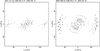 |
Fig. 1 TANAMI S band (u, υ) coverage in the most extended array configuration for sources of low and high declination. Due to the geographical layout of the array at the southern hemisphere, we do not have antenna pairs that cover intermediate-length baselines. |
Summary of observing sessions and participating antennas.
3 Results
We have summarized the properties of the 26 targets and two calibrators included in the first three S-band observational epochs in Table A.1. The table displays the source designation and common name, the source class, and redshift. These observations are focused on the TeV sample, but one neutrino source, 1424–418, was also added to these sessions. Of the 26 sources, 10 have previously been studied in the X-band by the TANAMI team, and so references to these papers are also shown.
Based on the parameters of the modelfit components, we can calculate the brightness temperature, Tb,obs, of the core components in the following way (Kovalev et al. 2005):
![Mathematical equation: ${T_{{\rm{b}},{\rm{obs}}}}[{\rm{K}}] = 1.22 \times {10^{12}}\left( {{{{S_v}} \over {{\rm{Jy}}}}} \right){\left( {{v \over {{\rm{GHz}}}}} \right)^{ - 2}}{\left( {{{{b_{{\rm{min}}}} \times {b_{{\rm{maj}}}}} \over {{\rm{ma}}{{\rm{s}}^2}}}} \right)^{ - 1}}(1 + z),$](/articles/aa/full_html/2024/01/aa47823-23/aa47823-23-eq1.png) (1)
(1)
where Sv is the flux density of the component, v is the observing frequency, and bmin and bmaj are the minor and major axes of the component. Errors in flux density are estimated to be 10% (Ojha et al. 2010) and errors of the component sizes are taken as one-fifth of the beam minor axis (Lister et al. 2009). We computed the resolution limit based on Eq. (2) of Kovalev et al. (2005), and found that all components are resolved (see Table A.3). The characteristics of the clean hybrid images are summarized in Table A.3 for the TeV sample and in Table A.2 for additional sources. The source structure is described in Col. 2; Col. 3 shows the observing epoch, and Cols. 4–8 show the clean image properties including beam major and minor axis, position angle, total flux density, rms noise level, and the lowest contours used in the clean images in Figs. 2 and 3. Columns 9-11 describe the flux density, size, and brightness temperature of the core components, and Cols. 12 and 13 display the HE properties of the source.
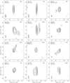 |
Fig. 2 Clean maps of the TANAMI TeV sample at 2.3 GHz. Image properties are summarized in Table A.3. Lowest contours are listed in Table A.3, and contour levels increase by a factor of two. The class is given in the top right corner of the image (see Table A.1). |
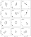 |
Fig. 3 Clean maps of the TANAMI TeV sample at 2.3 GHz, continuing Fig. 2. Lowest contours are listed in Table A.3, and contour levels increase by a factor of two. The class is given in the top right corner of the image (see Table A.1). |
4 Notes on individual sources
In this section, we provide a short summary of previous results from the literature regarding each of the sources of our TeV-sample and describe the source morphology in our observations.
0011–191. 8.4 GHz observations of Piner & Edwards (2014) with the VLBA reveal a compact core–jet structure with an opening angle of 26.2°. The jet component is close to stationary at ~1 mas (Piner & Edwards 2018a). Our 2.3 GHz images reveal a faint, compact core structure with a flux density of 140 mJy.
0031–196. This source is part of the HBL sample presented in Piner & Edwards (2014). It shows an extended jet on par-sec scales that has a proper motion of 0.204 ± 0.071 mas yr−1 and an opening angle of 18.2°. The source was detected at VHE by H.E.S.S. (Abdalla et al. 2020). Our images show only a core with a flux density of 200 mJy, because we lack the sensitivity to detect the extended jet emission.
0236–314. This is an X-ray source from the ROSAT Bright Survey (Schwope et al. 2000), and has been detected by Fermi in 2FGL (Ackermann et al. 2011) and H.E.S.S. (Gaté et al. 2017) as well. The TANAMIS band image shows a single-sided core–jet structure.
0301–243. The source was monitored by MOJAVE at 15 GHz between 2010 and 2012. Superluminal apparent speeds of up to 2.3 ± 0.5 c were detected (Lister et al. 2019). Both the 15 GHz MOJAVE and 22 and 43 GHz (Piner & Edwards 2023) observations show an unresolved core and an extended jet towards the southwest. We recover a similar structure with an extended jet reaching ~30 mas. The source is part of the Fermi Bright Source List (Abdo et al. 2009a), and has been detected by H.E.S.S. (H.E.S.S. Collaboration 2013b) with a 9.4σ significance and a flux of 1.4% of that of the Crab Nebula.
0347–121. This source shows a compact structure with a faint jet at 8.4 GHz (Piner & Edwards 2014), similar to what we see in the S band. The opening angle is measured to be 21.6°, and apparent speeds of 1.7 ± 1.2 c are detected by Piner & Edwards (2018a). A VHE detection by H.E.S.S. reveals an integral flux of 0.02 Crab units (CU) above 250 GeV and a power-law spectrum with Γ = 3.10 ± 0.33 between 250 GeV and 3 TeV (Aharonian et al. 2007b). The SED can be reasonably described by a one-zone model (Aharonian et al. 2007b).
0426–380. This source is currently the furthest known VHE-emitting FSRQ at ɀ = 1.1 (Tanaka et al. 2013), and has been part of the TANAMI X-band sample since 2009; the first images were published in Müller et al. (2018). 0426–380 shows a core–jet structure with the jet pointing west–southwest.
0447–439. This source is a Fermi Bright Source List blazar (Abdo et al. 2009a) and has been detected at VHE (H.E.S.S. Collaboration 2013a) with an integrated flux density of 0.03 CU. 0447–439 shows a faint extended jet towards the northwest, both in S - and X-band (Müller et al. 2018).
0548–322. This source resides in a giant elliptical galaxy in the center of Abell S0549 (Falomo et al. 1995). 0548–322 has also been observed by Piner & Edwards (2013) and Piner & Edwards (2014) at 8 and 15 GHz. These observations reveal an unresolved core and a faint jet pointing towards the northeast with an opening angle of 13.4°. On the other hand, our 2.3 GHz observations show only the core – with a flux density of 30 mJy –due to the low image sensitivity.
0625–354. This is an FR I radio galaxy hosted by a giant elliptical galaxy in the center of Abell 3392. First TANAMI images of the source at 8.4GHz were published in Ojha et al. (2010). Based on a kinematic analysis of nine epochs, Angioni et al. (2019) found superluminal motions with apparent speeds reaching ~3 c from the radio core. In the S band, the jet extends ~20 mas to the southeast, but tapered images of Ojha et al. (2010) reveal a jet up to 40 mas. Among many other FR I radio galaxies, 0625-354 has also been detected at VHE (H.E.S.S. Collaboration 2018) with an integral flux of 0.04 CU and a photon index of Γ = 2.8 ± 0.5.
0903–573. This source was first detected in the GeV range by Fermi LAT in 2015 (Carpenter & Ojha 2015). The source was considered a blazar candidate of unknown type until recently, when it was classified as a BL Lac object by Lefaucheur & Pita (2017). 0903–573 exhibited a complex γ-ray flaring activity during 2018 and 2020 (Mondal et al. 2021), which coincides with our first S -band observation. Our image reveals a core and an extended jet in the northwest direction.
1008–310. X band observations of Piner & Edwards (2014) and Piner & Edwards (2018a) show a compact core structure with a faint jet with an opening angle of 47.8°. Our 2.3 GHz image shows a slightly more extended jet towards the east–northeast. Integral flux above 0.2 TeV is 0.008 CU (H.E.S.S. Collaboration 2012).
1101–232. This source is hosted by an elliptical host galaxy. On kiloparsec scales, it shows a one-sided structure with a diffuse extension to the north (Laurent-Muehleisen et al. 1993). Observations at 5 and 8 GHz with the VLBA (Tiet et al. 2012), as well as our 2.3 GHz TANAMI observations, show a core with a faint, slightly extended jet to the northwest. Aharonian et al. (2007a) detected the source at VHE with H.E.S.S. Yan et al. (2012) showed that SED modeling can recover the observed TeV emission by using slightly beamed HE jet emission, but only the models with moderately high Doppler factors result in a jet in equipartition. Yan et al. (2012) suggest that inverse Compton scattering of the cosmic microwave background (CMB) photons in the extended jet is the main source of the TeV emission.
1253–053. 3C 279 is one of the most well-studied AGN in VLBI science and has been monitored by MOJAVE at 15 GHz since 1995, and by the Boston University Blazar Group at 43 GHz since 2007. On VLBI scales, the jet has a well-collimated one-sided structure, which is similar to our findings from S -band images, but on kiloparsec scales it shows a significant bend towards the east (Cheung 2002). RadioAstron observations at 22 GHz reveal a filamentary structure in the jet interpreted as Kelvin–Helmholtz instability (Fuentes et al., in prep.). Event Horizon Telescope (EHT) observations at 230 GHz show two components within the inner 150 µas of the 86 GHz core, with the upstream feature identified as the core oriented perpendicular to the downstream jet component (Kim et al. 2020). The core features show apparent speeds of ~15–20 c, which are consistent with values measured at centimeter wavelengths. 3C 279 was the first blazar detected in the γ-rays (Hartman et al. 1992), and has since been detected at VHE by MAGIC as well (MAGIC Collaboration 2008). The source has also been noted as a possible source of astrophysical neutrinos (Plavin et al. 2020).
1312–423. This source was detected by H.E.S.S. (H.E.S.S. Collaboration 2013c) and shown to have an integral flux density of 0.5% of that of the Crab Nebula. With the careful modeling of Cen A, these authors recover the source in the HE Fermi LAT data as well. Our S -band observations show a core and a slight extension of the jet towards the northeast.
1322–428. Cen A is an FR I radio galaxy (Tingay et al. 1998), and is the closest radio-loud AGN to the Earth. The source was detected early on by Fermi LAT and is part of the Fermi Bright Source List (Abdo et al. 2009a). The first X-band TANAMI image of Cen A was published in Ojha et al. (2010), which was followed by a detailed analysis of the source by Müller et al. (2014). The jet shows differential motion, that is to say, downstream features exhibit higher velocities than those closer to the VLBI core. This observation leads the authors to propose a spine-sheath structure present in the jet, which has been detected on subparsec scales at 230 GHz with the EHT (Janssen et al. 2021). Based on the jet–counterjet ratio, the viewing angle is constrained to fall between 12° and 45°. Our S -band images also show a double-sided structure with an extended, well-collimated jet.
1440–389. Müller et al. (2018) presented 8.4 GHz images of this source from TANAMI. The source shows a compact structure in S band with a jet that can be modeled by a single component. 1440–389 was first detected at VHE in 2012 (Abdalla et al. 2020), and was recently detected in a high γ-state by the Fermi LAT for the first time (Ciprini et al. 2022).
1510–089. This source has been part of the MOJAVE program since 1995, but observations were dropped in 2013, and then taken up again recently in 2021. On parsec scales, the jet shows a one-sided structure, which we also recover in our 2.3 GHz images. The MOJAVE kinematic analysis (Lister et al. 2019) shows maximum apparent speeds up to 28.0 ± 0.6 c, which suggests highly beamed emission (Liodakis et al. 2017). Multifrequency radio observations during high states in 2015–2017 reveal the emergence of two new jet components almost cotemporal to the HE flares; during one of the flares, the jet showed a limb-brightened linear polarization structure in the core region (Park et al. 2019). The authors conclude that the passing of the new components through stationary shocks gives rise to the γ-ray emission, and that the jet shows a complex transverse velocity structure that changes with time (MacDonald et al. 2015; Casadio et al. 2017).
1514–241. AP Librae has been part of MOJAVE between 1997 and 2012. Observations at 15 GHz show a 30 mas extended jet with a complex structure. In S band, we recover a double-sided jet. The maximum jet speed from MOJAVE observations is 6.21 ± 0.26 c (Lister et al. 2019). If we assume Doppler factors above 10, this suggests the jet viewing angle falls below 5° (Lister et al. 2013). Given the superluminal apparent jet speed and the small viewing angle, the double-sided jet structure in the S band image is of interest. VHE detection was reported by H.E.S.S. Collaboration (2015) with H.E.S.S. The VHE emission has been proposed to originate from the extended jet – which is also detected in the X-rays – via inverse Compton scattering of the CMB photons (Zacharias & Wagner 2016).
1515–273. TXS 1515–273 was detected by MAGIC (Acciari et al. 2021) during a γ-ray flare by Fermi (Cutini 2019). MOJAVE images reveal a one-sided jet structure that can be modeled as one component with an apparent speed of 0.73 ± 0.18 c (Lister et al. 2021). Our S -band images also show a core–jet morphology pointing toward the east.
1600–489. First 8.4-GHz TANAMI observations of this object were published in Müller et al. (2014). The source shows a double-sided structure, and due to its nonblazar-like spectral properties, it is classified as a compact symmetric object (CSO). The source is bright in the γ-rays (Abdo et al. 2009a). Our new S -band images show a double-sided jet structure and bright central core, which is reminiscent of the CSO class.
2005–489. This source was the first blazar independently detected by H.E.S.S. at VHE, and the second source noted as a VHE emitter in the southern hemisphere (Aharonian et al. 2005b). The integral flux is 0.025 of that of the Crab Nebula and has a very soft spectrum with a photon index of Γ = 4.0 ± 0.4. Both X-band TANAMI observations by Ojha et al. (2010) and our new 2.3 GHz image show an elongated core in the northeast–southwest direction and a diffuse jet emission to the southwest.
2155–304. 15 GHz VLBA (Piner & Edwards 2004; Piner et al. 2010), 8 GHz and 22 GHz TANAMI observations (Ojha et al. 2010), and our new 2.3 GHz image reveal an initially well-collimated jet on mas scales. The first polarimetric image published by (Piner et al. 2008) reveals polarization in the core region with a polarization fraction of 2.9% and EVPAs with a position angle of 131° misaligned with the jet position angle by 30°. The source 2155–304 was detected at VHE in 1999 by the University of Durham Mark 6 atmospheric Cherenkov telescope (Chadwick et al. 1999), and can exhibit integral fluxes of up to 60% of that of the Crab Nebula (Aharonian et al. 2005a). The source exhibited a high flaring activity during 2006, when Doppler factors over 100 were used to model the SED (Aharonian et al. 2007c), which is much higher than typical Doppler factors estimated from VLBI data.
2322–409. While observing PKS 2316–423, Abdalla et al. (2019) detected an excess in hard γ-rays at the position of 1ES 2322–409 with H.E.S.S. The VHE spectrum can be described with a power law with the soft photon index of Γ = 3.40 ± 0.86. The only published VLBI image of the source is presented by Schinzel et al. (2017) with the VLBA at 7.62GHz. The source has a jet extending ~ 4 mas towards the northeast. Our S band image shows a similar morphology, but the jet points towards east.
2356–309. This source has been reported as an extreme synchrotron peaked blazar because its low-energy SED component peaks in the X-rays (Costamante et al. 2001). VLBI observations of Tiet et al. (2012) at 5 and 8 GHz show a core and a jet extending a few mas from the core. Our new TANAMI images reveal a similar structure.
5 Discussion
The morphology of radio-loud AGN can be described as double-sided when we detect both the jet and the counter-jet, single-sided when we only see the jet, or as compact cores without jet emission (Kellermann et al. 1998). Of the sources in the sample, 25% show only the radio core, 62.5% are single-sided, and the rest only exhibit double-sided jets. Faint S2.3 GHz < 50 mJy sources on average show no extended jet emission, because the low signal-to-noise ratio prohibits the robust detection of jet emission. With that said, nine targets have total flux densities below 50 mJy, and only five reach 1 Jy.
The upper left-hand panel of Fig. 4 shows the redshift distribution of the TANAMI TeV sources. While the distribution of HBL and EHBL objects peaks around ɀ ~ 0.1, FSRQs in the sample fall between ɀ ~ 0.36 and 1.11, and 0426–380 at ɀ = 1.11 is the furthest known TeV emitter to date (Tanaka et al. 2013). The distribution of BL Lacs and FSRQs is consistent with the redshift distribution seen in the Bright AGN Source List (Abdo et al. 2009b) – which is a γ-ray-selected sample –, where BLLacs are mainly located below a redshift of 0.5, and the distribution of FSRQs peaks around ɀ ~ 1. However, the redshift distribution of TeV-detected AGN is biased for several reasons. The current generation of Imaging Atmospheric Cherenkov Telescopes (IACTs) operate in pointing mode, which means that they lack full-sky coverage. In addition, most AGN observed at VHE are only detected during high states of activity because of the lack of sensitivity of IACTs. Nevertheless, these issues will be overcome with the arrival of the Cherenkov Telescope Array (Actis et al. 2011). TeV emission from high-redshift sources is also affected by the attenuation from the extragalactic background light. In addition, many BL Lac objects have no redshifts available, which is due to the lack of detectable emission lines in their spectra, especially when considering high-redshift sources, further decreasing the number of known distant TeV-emitting AGN (Sol 2018).
The logarithmic GeV γ-ray photon flux distribution (Fig. 4, upper right panel) shows that BL Lac objects are distributed evenly, but mainly inhabit the fainter end of the sample. In addition, γ-ray brightness shows an inverse relation with the frequency of the synchrotron peak, that is, EHBL and HBL sources are dimmer at higher energies. The photon flux distribution of the Fermi-detected blazars from the above-mentioned Bright AGN Source List (Abdo et al. 2009b) peaks around 10−7 ph cm−2 s−1. However, our TeV sample shows a rather uniform distribution, with a mean photon flux of 9.09 × 10⁻⁹ ph cm−2 s−1.
The 2.3 GHz core brightness temperature distributions (Fig. 4, lower panels) show that BL Lac objects have the lowest Tb,core values, with a mean of 7.49 × 10⁹ K, and FSRQs exhibit the highest Tb,core values, with an average of 1.52 × 10¹⁰ K. This is also seen in the study of a complete flux-limited sample of AGN (Lister et al. 2011), where HBL sources show lower brightness temperatures than other BLLac objects and quasars. (Homan et al. 2021) reported that BLLac objects in this flux-limited sample show the same trend that we find for our TeV-detected sample, namely that there is an inverse relation between the synchrotron peak frequency and the median core brightness temperature.
The Tb,core distribution with γ-ray flux classes marked shows that γ-ray-low (Sγ < 10−9 ph cm−2 s−1) objects tend to exhibit lower core brightness temperatures, while medium (10−9 < Sγ < 10−8 ph cm−2 s−1) and bright (>10−8 ph cm−2 s−1) sources have higher Tb,core values. A similar trend is recovered for the above-mentioned MOJAVE 1.5-Jy flux-limited sample, in which quasars show higher median core brightness temperatures and are more luminous at GeV energies than BL Lacs (Homan et al. 2021). These results suggest that the emission from low-synchrotron-peaked objects, like FSRQs and LBLs, is more strongly Doppler boosted than that from high-synchrotron-peaked objects, such as HBL and EHBL sources.
The average and median Tb,core for the TANAMI TeV sample are 8.19 × 10¹⁰ K and 4.9 × 10⁹ K, respectively. Twenty-one Tb,core values are below the equipartition brightness temperature of Teq ≈ 5 × 10¹⁰ K (Readhead 1994) and all but one of the values fall below the inverse Compton catastrophe limit of ≈ 1012 K (Kellermann & Pauliny-Toth 1969). This suggests that, in most cases, the emission from these sources is not beamed at 2.3 GHz. Observations at 15 GHz in MOJAVE, a sample dominated by LBL and FSRQ objects, reveal a mean core brightness temperature of 2.93 × 10¹¹ K with a median of 3.66 × 10¹¹ K (Homan et al. 2021), which is significantly higher than those observed in our sample. Tb,core values of the X-band TANAMI sample from Böck et al. (2016) have an average and median of 9.62 × 10¹¹ K and 2.1 × 10¹¹ K, respectively, which are consistent with those of the MOJAVE sample. The nearly one-order-of-magnitude lower average Tb,core for the TeV sample has been shown as a characteristic of VHE-detected sources (Piner & Edwards 2018b).
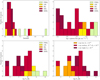 |
Fig. 4 Histogram showing the redshift (upper left panel), 0.1–100 GeV photon flux (upper right panel), and 2.3-GHz core brightness temperature (lower panels) distribution of sources in the TeV sample. |
6 Conclusion
In this work, we present the first results of our new 2.3 GHz AGN monitoring, including all 24 TeV-detected sources at the southern hemisphere at the time of the observations. The 2.3 GHz band was added in our program to better study extended jet emission and to include TeV sources in our sample that would be too faint to detect at higher frequencies. With the inclusion of Parkes and ATCA, we were capable of detecting even the faintest (S2.3G Hz ≈ 10 mJy) target in the sample. While this was a success, the current long transoceanic baselines to the Hartebeesthoek antenna yield only limited sensitivity, which degrades the image fidelity and angular resolution in observations of faint targets. This is a strong limitation for studies of the bulk of the HBL and extreme-blazar population. In order to improve our observations, we support the efforts to phase up the MeerKAT array, with which we would be able to achieve three times better sensitivity on the long baselines.
We fitted circular Gaussian components to model the source structures and calculated the brightness temperatures for the radio core. Core brightness temperature distributions reveal that the FSRQs in the sample generally have higher core brightness temperatures than BL Lacs and radio galaxies. We also observe that, with increasing γ-ray photon flux, core brightness temperatures are higher as well. Comparing this sample to 8.4 GHz TANAMI and 15 GHz MOJAVE results, which are samples dominated by FSRQs and low-synchrotron-peaked objects, we find that the Tb,core values in the S band are up to one magnitude lower than average values in the other samples, which is consistent with previous results of Piner & Edwards (2018b), who noted that TeV-detected sources have lower Tb,core. However, at low frequencies, it is also possible that we do not detect the optically thick VLBI core, but instead only a bright, optically thin jet component that we identify as the core. As brightness temperature measurements are heavily dependent on the maximum baseline length and the flux density of the component, bright jet features, like the core, can exhibit high Tb values.
Due to the success of the first three S band observing epochs, we continue to monitor VHE-detected AGN and perform kinematic and spectral studies once a sufficient number of observing epochs is reached. While the 2.3 GHz observations lack the resolution and sensitivity to determine the location of the γ-ray production or to differentiate between jet models suggested to resolve the Doppler crisis, they enable us to study the faintest Te V-emitters and to perform multi-frequency studies together with our 8.4 GHz monitoring. TANAMI is currently the only AGN monitoring program on the southern hemisphere, and forming complete samples to study these rarely observed targets is crucial in order to advance multiwavelength studies.
Acknowledgements
The authors would like to thank the anonymous referee for their valuable comments on the manuscript. We thank H. Müller for his constructive suggestions to improve our work. The Long Baseline Array is part of the Australia Telescope National Facility (https://ror.org/05qajvd42) which is funded by the Australian Government for operation as a National Facility managed by CSIRO. From the 2023 July 1, operation of Warkworth was transferred from AUT University to Space Operations New Zealand Ltd with new funding from Land Information New Zealand (LINZ). This research was supported through a PhD grant from the International Max Planck Research School (IMPRS) for Astronomy and Astrophysics at the Universities of Bonn and Cologne. M2FINDERS project has received funding from the European Research Council (ERC) under the European Union’s Horizon 2020 research and innovation programme (grant agreement no. 101018682). M.K. and F.R. acknowledge funding by the Deutsche Forschungsgemeinschaft (DFG, German Research Foundation) – grant 434448349.
Appendix A Additional data
Sources observed during the first three S band epochs.
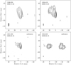 |
Fig. A.1 Clean maps of additional sources and calibrators included in the 2.3 GHz observations. Image parameters and lowest contours are listed in Table A.2. Contour levels increase by a factor of two. |
Image properties of non-TeV sources and calibrators observed during 2020–2021 in S band.
Image properties of the TeV-detected AGN in our observations.
References
- Abdalla, H., Aharonian, F., Ait Benkhali, F., et al. 2019, MNRAS, 482, 3011 [Google Scholar]
- Abdalla, H., Adam, R., Aharonian, F., et al. 2020, MNRAS, 494, 5590 [NASA ADS] [CrossRef] [Google Scholar]
- Abdo, A. A., Ackermann, M., Ajello, M., et al. 2009a, ApJS, 183, 46 [NASA ADS] [CrossRef] [Google Scholar]
- Abdo, A. A., Ackermann, M., Ajello, M., et al. 2009b, ApJ, 700, 597 [CrossRef] [Google Scholar]
- Abdo, A. A., Ackermann, M., Agudo, I., et al. 2010, ApJ, 716, 30 [NASA ADS] [CrossRef] [Google Scholar]
- Abdollahi, S., Acero, F., Baldini, L., et al. 2022, ApJS, 260, 53 [NASA ADS] [CrossRef] [Google Scholar]
- Acciari, V. A., Ansoldi, S., Antonelli, L. A., et al. 2021, MNRAS, 507, 1528 [NASA ADS] [CrossRef] [Google Scholar]
- Ackermann, M., Ajello, M., Allafort, A., et al. 2011, ApJ, 743, 171 [Google Scholar]
- Actis, M., Agnetta, G., Aharonian, F., et al. 2011, Exp. Astron., 32, 193 [NASA ADS] [CrossRef] [Google Scholar]
- Aharonian, F., Akhperjanian, A. G., Aye, K.-M., et al. 2005a, A&A, 430, 865 [CrossRef] [EDP Sciences] [Google Scholar]
- Aharonian, F., Akhperjanian, A. G., Aye, K.-M., et al. 2005b, A&A, 436, L17 [NASA ADS] [CrossRef] [EDP Sciences] [Google Scholar]
- Aharonian, F., Akhperjanian, A. G., Bazer-Bachi, A. R., et al. 2007a, A&A, 470, 475 [NASA ADS] [CrossRef] [EDP Sciences] [Google Scholar]
- Aharonian, F., Akhperjanian, A. G., Barres de Almeida, U., et al. 2007b, A&A, 473, L25 [NASA ADS] [CrossRef] [EDP Sciences] [Google Scholar]
- Aharonian, F., Akhperjanian, A. G., Bazer-Bachi, A. R., et al. 2007c, ApJ, 664, L71 [NASA ADS] [CrossRef] [Google Scholar]
- Aleksić, J., Alvarez, E. A., Antonelli, L. A., et al. 2012, A&A, 542, A100 [NASA ADS] [CrossRef] [EDP Sciences] [Google Scholar]
- Angioni, R., Ros, E., Kadler, M., et al. 2019, A&A, 627, A148 [NASA ADS] [CrossRef] [EDP Sciences] [Google Scholar]
- Arsioli, B., Fraga, B., Giommi, P., et al. 2015, A&A, 579, A34 [NASA ADS] [CrossRef] [EDP Sciences] [Google Scholar]
- Atwood, W. B., Abdo, A. A., Ackermann, M., et al. 2009, ApJ, 697, 1071 [CrossRef] [Google Scholar]
- Böck, M., Kadler, M., Müller, C., et al. 2016, A&A, 590, A40 [NASA ADS] [CrossRef] [EDP Sciences] [Google Scholar]
- Böttcher, M., & Els, P. 2016, ApJ, 821, 102 [CrossRef] [Google Scholar]
- Carpenter, B., & Ojha, R. 2015, ATel, 7704 [Google Scholar]
- Casadio, C., Krichbaum, T., Marscher, A., et al. 2017, Galaxies, 5, 67 [NASA ADS] [CrossRef] [Google Scholar]
- Chadwick, P. M., Lyons, K., McComb, T. J. L., et al. 1999, ApJ, 513, 161 [NASA ADS] [CrossRef] [Google Scholar]
- Chang, Y.-L., Arsioli, B., Giommi, P., et al. 2019, A&A, 632, A77 [NASA ADS] [CrossRef] [EDP Sciences] [Google Scholar]
- Cheung, C. C. 2002, ApJ, 581, L15 [NASA ADS] [CrossRef] [Google Scholar]
- Ciprini, S., Cheung, C. C., & Fermi Large Area Telescope Collaboration 2022, ATel, 15635 [Google Scholar]
- Costamante, L., Ghisellini, G., Giommi, P., et al. 2001, A&A, 371, 512 [NASA ADS] [CrossRef] [EDP Sciences] [Google Scholar]
- Craig, N., & Fruscione, A., 1997, AJ, 114, 1356 [NASA ADS] [CrossRef] [Google Scholar]
- Cutini, S. 2019, ATel, 12532 [Google Scholar]
- Falomo, R., Pesce, J. E., & Treves, A. 1995, ApJ, 438, L9 [NASA ADS] [CrossRef] [Google Scholar]
- Ganguly, R., Lynch, R. S., Charlton, J. C., et al. 2013, MNRAS, 435, 1233 [NASA ADS] [CrossRef] [Google Scholar]
- Gaté, F., H.E.S.S. Collaboration, & Fitoussi, T. 2017, 35th International Cosmic Ray Conference (ICRC2017), 301, 645 [Google Scholar]
- Georganopoulos, M., & Kazanas, D. 2003, ApJ, 594, L27 [NASA ADS] [CrossRef] [Google Scholar]
- Ghisellini, G., Tavecchio, F., & Chiaberge, M. 2005, A&A, 432, 401 [CrossRef] [EDP Sciences] [Google Scholar]
- Giannios, D., Uzdensky, D. A., & Begelman, M. C. 2009, MNRAS, 395, L29 [NASA ADS] [CrossRef] [Google Scholar]
- Goldoni, P., Pita, S., Boisson, C., et al. 2016, A&A, 586, A2 [NASA ADS] [CrossRef] [EDP Sciences] [Google Scholar]
- Greisen, E. W. 2003, Information Handling in Astronomy – Historical Vistas (Dordrecht: Kluwer Academic Publishers), 285, 109 [CrossRef] [Google Scholar]
- Gulyaev, S., Natusch, T., & Wilson, D. 2010, Sixth International VLBI Service for Geodesy and Astronomy. Proceedings from the 2010 General Meeting, 113 [Google Scholar]
- Hartman, R. C., Bertsch, D. L., Fichtel, C. E., et al. 1992, ApJ, 385, L1 [Google Scholar]
- H.E.S.S. Collaboration (Abramowski, A., et al.) 2012, A&A, 542, A94 [NASA ADS] [CrossRef] [EDP Sciences] [Google Scholar]
- H.E.S.S. Collaboration (Abramowski, A., et al.) 2013a, A&A, 552, A118 [NASA ADS] [CrossRef] [EDP Sciences] [Google Scholar]
- H.E.S.S. Collaboration (Abramowski, A., et al.) 2013b, A&A, 559, A136 [NASA ADS] [CrossRef] [EDP Sciences] [Google Scholar]
- H.E.S.S. Collaboration (Abramowski, A., et al.) 2013c, MNRAS, 434, 1889 [NASA ADS] [CrossRef] [Google Scholar]
- H.E.S.S. Collaboration (Abramowski, A., et al.) 2015, A&A, 573, A31 [NASA ADS] [CrossRef] [EDP Sciences] [Google Scholar]
- H.E.S.S. Collaboration (Abdalla, H., et al.) 2018, MNRAS, 476, 4187 [NASA ADS] [CrossRef] [Google Scholar]
- Homan, D. C., Cohen, M. H., Hovatta, T., et al. 2021, ApJ, 923, 67 [NASA ADS] [CrossRef] [Google Scholar]
- Jackson, C. A., Wall, J. V., Shaver, P. A., et al. 2002, A&A, 386, 97 [NASA ADS] [CrossRef] [EDP Sciences] [Google Scholar]
- Janssen, M., Falcke, H., Kadler, M., et al. 2021, Nat. Astron., 5, 1017 [NASA ADS] [CrossRef] [Google Scholar]
- Jones, D. H., Read, M. A., Saunders, W., et al. 2009, MNRAS, 399, 683 [Google Scholar]
- Jorstad, S. G., Marscher, A. P., Smith, P. S., et al. 2013, ApJ, 773, 147 [Google Scholar]
- Keeney, B. A., Stocke, J. T., Pratt, C. T., et al. 2018, ApJS, 237, 11 [NASA ADS] [CrossRef] [Google Scholar]
- Kellermann, K. I., & Pauliny-Toth, I. I. K. 1969, ApJ, 155, L71 [NASA ADS] [CrossRef] [Google Scholar]
- Kellermann, K. I., Vermeulen, R. C., Zensus, J. A., et al. 1998, AJ, 115, 1295 [NASA ADS] [CrossRef] [Google Scholar]
- Kim, J.-Y., Krichbaum, T. P., Broderick, A. E., et al. 2020, A&A, 640, A69 [EDP Sciences] [Google Scholar]
- Kovalev, Y. Y., Kellermann, K. I., Lister, M. L., et al. 2005, AJ, 130, 2473 [Google Scholar]
- Lavaux, G., & Hudson, M. J. 2011, MNRAS, 416, 2840 [Google Scholar]
- Lauer, T. R., Postman, M., Strauss, M. A., et al. 2014, ApJ, 797, 82 [Google Scholar]
- Laurent-Muehleisen, S. A., Kollgaard, R. I., Moellenbrock, G. A., et al. 1993, AJ, 106, 875 [NASA ADS] [CrossRef] [Google Scholar]
- Lefaucheur, J., & Pita, S. 2017, A&A, 602, A86 [NASA ADS] [CrossRef] [EDP Sciences] [Google Scholar]
- Lico, R., Giroletti, M., Orienti, M., et al. 2012, A&A, 545, A117 [CrossRef] [EDP Sciences] [Google Scholar]
- Liodakis, I., Zezas, A., Angelakis, E., et al. 2017, A&A, 602, A104 [NASA ADS] [CrossRef] [EDP Sciences] [Google Scholar]
- Lister, M. L., Cohen, M. H., Homan, D. C., et al. 2009, AJ, 138, 1874 [NASA ADS] [CrossRef] [Google Scholar]
- Lister, M. L., Aller, M., Aller, H., et al. 2011, ApJ, 742, 27 [CrossRef] [Google Scholar]
- Lister, M. L., Aller, M. F., Aller, H. D., et al. 2013, AJ, 146, 120 [Google Scholar]
- Lister, M. L., Homan, D. C., Hovatta, T., et al. 2019, ApJ, 874, 43 [NASA ADS] [CrossRef] [Google Scholar]
- Lister, M. L., Homan, D. C., Kellermann, K. I., et al. 2021, ApJ, 923, 30 [NASA ADS] [CrossRef] [Google Scholar]
- MacDonald, N. R., Marscher, A. P., Jorstad, S. G., et al. 2015, ApJ, 804, 111 [NASA ADS] [CrossRef] [Google Scholar]
- MAGIC Collaboration (Albert, J., et al.) 2008, Science, 320, 1752 [NASA ADS] [CrossRef] [Google Scholar]
- Mannheim, K. 1993, A&A, 269, 67 [NASA ADS] [Google Scholar]
- Mao, L. S. 2011, New Astron., 16, 503 [NASA ADS] [CrossRef] [Google Scholar]
- Maraschi, L., Ghisellini, G., & Celotti, A. 1992, ApJ, 397, L5 [CrossRef] [Google Scholar]
- Marscher, A. P., Jorstad, S. G., Agudo, I., et al. 2012, ArXiv e-prints [arXiv:1204.6707] [Google Scholar]
- Mondal, S. K., Prince, R., Gupta, N., et al. 2021, ApJ, 922, 160 [NASA ADS] [CrossRef] [Google Scholar]
- Müller, C., Kadler, M., Ojha, R., et al. 2014, A&A, 569, A115 [NASA ADS] [CrossRef] [EDP Sciences] [Google Scholar]
- Müller, C., Kadler, M., Ojha, R., et al. 2018, A&A, 610, A1 [NASA ADS] [CrossRef] [EDP Sciences] [Google Scholar]
- Neeleman, M., Prochaska, J. X., Ribaudo, J., et al. 2016, ApJ, 818, 113 [Google Scholar]
- Ojha, R., Fey, A. L., Johnston, K. J., et al. 2004, AJ, 127, 1977 [NASA ADS] [CrossRef] [Google Scholar]
- Ojha, R., Kadler, M., Böck, M., et al. 2010, A&A, 519, A45 [NASA ADS] [CrossRef] [EDP Sciences] [Google Scholar]
- Park, J., Lee, S.-S., Kim, J.-Y., et al. 2019, ApJ, 877, 106 [Google Scholar]
- Paturel, G., Dubois, P., Petit, C., et al. 2002, LEDA [Google Scholar]
- Piner, B. G., & Edwards, P. G. 2004, ApJ, 600, 115 [Google Scholar]
- Piner, B. G., & Edwards, P. G. 2013, Eur. Phys. J. Web Conf., 61, 04021 [NASA ADS] [CrossRef] [EDP Sciences] [Google Scholar]
- Piner, B. G., & Edwards, P. G. 2014, ApJ, 797, 25 [NASA ADS] [CrossRef] [Google Scholar]
- Piner, B. G., & Edwards, P. G. 2018a, ApJ, 853, 68 [Google Scholar]
- Piner, B. G., & Edwards, P. G. 2018b, Fourteenth Marcel Grossmann Meeting – MG14 (World Scientific Publishing Co. Pte. Ltd.), 3074 [Google Scholar]
- Piner, B. G., & Edwards, P. G. 2023, https://whittierblazars.com/ [Google Scholar]
- Piner, B. G., Pant, N., & Edwards, P. G. 2008, ApJ, 678, 64 [Google Scholar]
- Piner, B. G., Pant, N., & Edwards, P. G. 2010, ApJ, 723, 1150 [Google Scholar]
- Plavin, A., Kovalev, Y. Y., Kovalev, Y. A., et al. 2020, ApJ, 894, 101 [NASA ADS] [CrossRef] [Google Scholar]
- Readhead, A. C. S. 1994, ApJ, 426, 51 [Google Scholar]
- Rieger, F. M., & Volpe, F. 2010, A&A, 520, A23 [NASA ADS] [CrossRef] [EDP Sciences] [Google Scholar]
- Saito, S., Stawarz, L., Tanaka, Y. T., et al. 2013, ApJ, 766, L11 [NASA ADS] [CrossRef] [Google Scholar]
- Schinzel, F. K., Petrov, L., Taylor, G. B., et al. 2017, ApJ, 838, 139 [CrossRef] [Google Scholar]
- Schwope, A., Hasinger, G., Lehmann, I., et al. 2000, Astron. Nachr., 321, 1 [NASA ADS] [CrossRef] [Google Scholar]
- Shepherd, M. C. 1997, Astronomical Data Analysis Software and Systems VI, A.S.P. Conference Series, 125, 77 [NASA ADS] [Google Scholar]
- Sol, H. 2018, J. Astrophys. Astron., 39, 52 [NASA ADS] [CrossRef] [Google Scholar]
- Tanaka, Y. T., Cheung, C. C., Inoue, Y., et al. 2013, ApJ, 777, L18 [NASA ADS] [CrossRef] [Google Scholar]
- Tavecchio, F., Becerra-Gonzalez, J., Ghisellini, G., et al. 2011, A&A, 534, A86 [CrossRef] [EDP Sciences] [Google Scholar]
- Thompson, D. J., Djorgovski, S., & de Carvalho, R. 1990, PASP, 102, 1235 [NASA ADS] [CrossRef] [Google Scholar]
- Tiet, V. C., Piner, B. G., & Edwards, P. G. 2012, ArXiv e-prints [arXiv:1205.2399] [Google Scholar]
- Tingay, S. J., Jauncey, D. L., Reynolds, J. E., et al. 1998, AJ, 115, 960 [NASA ADS] [CrossRef] [Google Scholar]
- Truebenbach, A. E., & Darling, J. 2017, ApJS, 233, 3 [CrossRef] [Google Scholar]
- Yan, D., Zeng, H., & Zhang, L. 2012, MNRAS, 424, 2173 [NASA ADS] [CrossRef] [Google Scholar]
- Zacharias, M., & Wagner, S. J. 2016, A&A, 588, A110 [NASA ADS] [CrossRef] [EDP Sciences] [Google Scholar]
All Tables
Image properties of non-TeV sources and calibrators observed during 2020–2021 in S band.
All Figures
|
Fig. 1 TANAMI S band (u, υ) coverage in the most extended array configuration for sources of low and high declination. Due to the geographical layout of the array at the southern hemisphere, we do not have antenna pairs that cover intermediate-length baselines. |
| In the text | |
|
Fig. 2 Clean maps of the TANAMI TeV sample at 2.3 GHz. Image properties are summarized in Table A.3. Lowest contours are listed in Table A.3, and contour levels increase by a factor of two. The class is given in the top right corner of the image (see Table A.1). |
| In the text | |
|
Fig. 3 Clean maps of the TANAMI TeV sample at 2.3 GHz, continuing Fig. 2. Lowest contours are listed in Table A.3, and contour levels increase by a factor of two. The class is given in the top right corner of the image (see Table A.1). |
| In the text | |
|
Fig. 4 Histogram showing the redshift (upper left panel), 0.1–100 GeV photon flux (upper right panel), and 2.3-GHz core brightness temperature (lower panels) distribution of sources in the TeV sample. |
| In the text | |
|
Fig. A.1 Clean maps of additional sources and calibrators included in the 2.3 GHz observations. Image parameters and lowest contours are listed in Table A.2. Contour levels increase by a factor of two. |
| In the text | |
Current usage metrics show cumulative count of Article Views (full-text article views including HTML views, PDF and ePub downloads, according to the available data) and Abstracts Views on Vision4Press platform.
Data correspond to usage on the plateform after 2015. The current usage metrics is available 48-96 hours after online publication and is updated daily on week days.
Initial download of the metrics may take a while.