| Issue |
A&A
Volume 674, June 2023
|
|
|---|---|---|
| Article Number | A168 | |
| Number of page(s) | 5 | |
| Section | Astrophysical processes | |
| DOI | https://doi.org/10.1051/0004-6361/202245171 | |
| Published online | 19 June 2023 | |
A discontinuity at the base of the transition layer located between the Keplerian accretion disk and the compact object
1
Dipartimento di Fisica, Università di Ferrara, Via Saragat 1, 44122 Ferrara, Italy
e-mail: titarchuk@fe.infn.it
2
Keldysh Institute of Applied Mathematics, Russian Academy of Sciences, 4 Miusskaya sq., Moscow, 125047
Russia
e-mail: kalasxel@gmail.com
Received:
8
October
2022
Accepted:
15
May
2023
Context. We study the geometry of the transition layer (TL) between the classical Keplerian accretion disk (the TL outer boundary) and the compact object at the TL inner boundary.
Aims. Our goal is to use the hydrodynamical formalism to demonstrate that the TL is created, together with a shock, in response to a discontinuity and to adjust the Keplerian disk motion to a central object (CO).
Methods. We apply hydrodynamical equations to describe a plasma motion near a CO in the TL.
Results. We point out that, before matter accretes to a CO, the TL cloud is formed between an adjustment radius and the TL inner boundary, which is probably a site where the emergent Compton spectrum originates. Using a generalization of the Randkine–Hugoniot relation and a solution of the azimutal force balance equation, we are able to reproduce the geometric characteristics of the TL.
Key words: accretion, accretion disks / radiation mechanisms: general / black hole physics / stars: neutron / white dwarfs
© The Authors 2023
 Open Access article, published by EDP Sciences, under the terms of the Creative Commons Attribution License (https://creativecommons.org/licenses/by/4.0), which permits unrestricted use, distribution, and reproduction in any medium, provided the original work is properly cited.
This article is published in open access under the Subscribe to Open model. Subscribe to A&A to support open access publication.
1. Introduction
Accretion onto compact objects, such as white dwarfs (WDs), neutron star (NSs), and black hole (BH) binaries, is very similar. The accreting matter, which has relatively large angular momentum, can form a disk or go to outflow (see Titarchuk et al. 2007; Shaposhnikov & Titarchuk 2009, hereafter TSA07, ST09, respectively). On the other hand, the plasma, which has low angular momentum, proceeds toward the compact object in almost a free-fall manner until the centrifugal force becomes sufficiently strong to halt the flow (see, e.g., Chakrabarti & Titarchuk 1995, hereafter CT95). There are therefore three definitive regions – a (Keplerian) disk, the shock, and a transition layer (TL) between the last stable orbit near a WD, NS, or BH and the shock –, and the emergent X-ray spectrum is likely formed within them. In this paper, we study the characteristics of the adjustment of the Keplerian disk flow to a central object (CO).
The disk starts to deviate from a Keplerian motion at a certain radius to adapt itself to the boundary conditions at the WD or NS surface (or at the last stable orbit, at r1 = 3rS, where rS is the Schwarzchild radius in the case of a BH). Titarchuk et al. (1998, hereafter TLM98) explained the millisecond variability detected by the Rossi X-Ray Timing Explorer (RXTE) in the X-ray emission from a number of low-mass X-ray binary systems (XRBs). Later, Seifina & Titarchuk (2010), Farinelli & Titarchuk (2011), and so on analyzed X-ray data from Sco X-1, 4U 1728−34, 4U 1608−522, 4U 1636−536, 4U 0614−091, 4U 1735−44, 4U 1820−30, and GX 5−1 in terms of dynamics of the centrifugal barrier, in a hot boundary region (the TL) surrounding a NS. These authors demonstrated that this region may experience relaxation oscillations and that the displacements of a gas element both in radial and vertical directions occur at the same main frequency, namely of the order of the local Keplerian frequency.
Observations of BH X-ray binaries and active galactic nuclei indicate that the accretion flows around BHs are composed of hot and cold gas. Both of them have been theoretically described in terms of a hot corona next to an optically thick, relatively cold disk. Liu & Qiao (2022; hereafter LQ22) reviewed the accretion flows around BHs with an emphasis on the physics that determines the configuration of hot and cold accreting gas, and how the configuration varies with the accretion rate and thereby produces various luminosities and spectra. These authors provide references to the famous solutions of the standard disk model, such as Shakura & Sunyaev (1973; hereafter SS73). The most successful applications of this model are the steady state and time-dependent nature of thin disks in dwarf novae and soft X-ray transients. Application of the four accretion models to BHs presented by LQ22 is constrained by both the theoretical assumption of specific models and observational luminosity and spectrum.
The soft photons from the innermost part of the disk are scattered off the hot electrons, forming the Comptonized X-ray spectrum (see Sunyaev & Titarchuk 1980, hereafter ST80). The electron temperature is regulated by the supply of soft photons from a disk, which depends on the ratio of the energy release (accretion rate) in a disk and the energy release in the TL. For example, the electron temperature is higher for lower accretion rates (see, e.g., CT95), while for a high accretion rate (of the order of the Eddington rate) the TL is cooled down very efficiently by the soft photon flux and the Comptonization. This is a possible mechanism for the low-frequency quasi-periodic oscillations (QPOs) discovered with the RXTE in a number of low-mass X-ray binary systems (LMXBs; see Strohmayer et al. 1996; van der Klis et al. 1996, hereafter S96 and VK96a, respectively; Zhang et al. 1996, TLM98, Titarchuk et al. 2007 hereafter TSA07). These observations reveal a wealth of high- and low-frequency X-ray variabilities that are believed to be due to the processes occurring in the very vicinity of an accreting NS and BH.
Lančová et al. (2019) discovered a new class of BH accretion disk solutions through 3D radiative magnetohydrodynamic simulations wherein the general relativity formalism is applied. These solutions combine features of thin, slim, and thick disk models, and provide a realistic description of BH disks and have a thermally stable, optically thick Keplerian region supported by magnetic fields. Mishra et al. (2020) conducted a detailed analysis of two-dimensional viscous radiation hydrodynamic numerical simulations of the Shakura–Sunyaev thin disks around a stellar mass BH, finding multiple robust, coherent oscillations occurring in the disk, including a trapped fundamental g-mode and standing-wave p-modes. This latter study suggests that these findings could be of astrophysical importance in the observed twin-peak high-frequency QPOs. Large-scale 3D magnetohydrodynamic simulations of accretion onto magnetized stars with tilted magnetic and rotational axes were run by Romanova et al. (2021), who showed that the inner parts of the disk become warped, tilted, and precess due to magnetic interaction between the magnetosphere and the disk. According to the results of numerical simulations by Lugovskii & Chechetkin (2012), large-scale instability in accretion disks reveals changes in a disk-flow structure because of the formation of large vortexes. Over time, this leads to the development of asymmetric spiral structures and results in angular-momentum redistribution within the disk.
Suková et al. (2017) conducted simulations of accretion flows with low angular momentum, filling the gap between spherically symmetric Bondi accretion and disk-like accretion flows. These authors identified ranges of parameters for which the shock, after formation, either moves toward or away from the central BH or for which a long-lasting oscillating shock is observed. The results are scalable with a central BH mass and can be compared to QPOs of selected microquasars and supermassive BHs in the centres of weakly active galaxies. In order to explain the evidence gathered by the NICER telescope for nondipolar magnetic field structures in rotation-powered millisecond pulsars, Das et al. (2022) conducted a suite of general relativistic magnetohydrodynamic simulations of accreting NSs for dipole, quadrupole, and quadrudipolar stellar field geometries. This study found that the location and size of the accretion columns resulting in hotspots change significantly depending on initial stellar field strength and geometry, providing a viable mechanism to explain the radio power in observed NS jets.
Despite the increasing role of numerical simulations of accretion, the consideration of relatively simple analytical models allows us to identify the response of the system to changes in a set of parameters, which in the case of numerical simulations becomes a very cumbersome task. In the present paper, we join other authors (e.g., Abramowicz & Fragile 2013; Ajay et al. 2022) in proposing a model of accretion onto a CO. We do this because existing models of shock waves (see e.g., Chakrabarti 1989) cannot correctly describe the abrupt transition between the accretion disk and the TL. Our goal is to construct a satisfactory model of the shock wave lying at the base of the TL that can correctly describe observational data for temperature and density (Seifina & Titarchuk 2010). In Sect. 2, we describe our approach to the TL model. In Sect. 3, we formulate equations to determine the vertical dependencies of density and pressure in the TL. In Sects. 4 and 5, we introduce the generalized Rankine–Hugoniot relation and take into account the rotation effect in the TL, respectively. We discuss our setup and final results in Sect. 6. Finally, we summarize our conclusions in Sect. 7.
2. Motivation and the model
Consideration of the two-dimensional structure of accretion disks is hampered by straightforward mathematical difficulties. Typically, a two-dimensional structure is only accounted for by an inhomogeneous distribution of matter within a layer of constant thickness 2h. Consideration of a disk of constant thickness is made possible by ignoring the vertical velocity vz. The more general case h = h(r) necessitates that we solve the equation dh/dr = (vz/u)|z = h(r), where u is the radial velocity, in order that we may describe the behavior of the height as the radius changes.
According to the observations and their interpretations (TLM98, ST09) the disk height may achieve very significant values near the TL, while at larger distances it is relatively small. The thermodynamic characteristics of the plasma change considerably: in the TL, its temperature can reach tens of keV and its density drops drastically (see e.g., ST09). This change is widely believed to be due to the presence of a shock wave (see e.g., CT95, TLM98 and ST09). Such a region near the CO is associated with the TL.
In an attempt to get closer to a two-dimensional consideration, we chose the following model to describe the shock (Fig. 1). The flow velocity is supposed to have only radial and azimuthal components on the both sides of the shock, both of which are independent of height. It is assumed that the height of the flow changes sharply by discontinuity from h2 (the disk thickness) to h1 (the TL thickness).
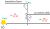 |
Fig. 1. Schematic representation of the considered model. |
We require the angular velocity ω of the TL to match the CO at its surface and to coincide with the disk velocity at the shock position r2. This angular velocity of the disk is supposed to be equal to the Keplerian velocity. Only the rϕ component of the viscous stress tensor is considered because it is responsible for removing the angular momentum. We consider the stress tensor form ηrωω′, where η is the turbulent viscosity.
The thermodynamic quantities of the flow have vertical dependencies, which are determined by the CO gravity and an equation of state. In order to identify them, we do not assume the smallness of the vertical coordinate compared to the radial one.
3. The vertical dependences
Let us start with the hydrostatic balance equation in the vertical direction:

where p and ρ are pressure and density and Φ is the gravitational potential created by the CO. We assume that the vertical distribution of matter is given by the polytropic relation p = Kρ1 + 1/n, where K is a constant related to the entropy and n is the polytropic index. Then the formal solution of Eq. (1) may be written as:

where  is an arbitrary function. We require the density and pressure to be zero at the inner boundary, z = ±h, and equal to some functions ρe, pe correspondingly at the equator z = 0. We then have:
Assuming the height is small compared to the radius |z|≪r, we may get the commonly used (Hōshi 1977; Matsumoto et al. 1984) dependence ρ = ρe(r)(1 − z2/h2)n. However, further on we did not assume that the height of TL is small compared to the radius.
We need integrals from such vertical dependences:
To the best of our knowledge, there is no general expression for such an integral for arbitrary n, but it may be calculated for particular values.
4. Generalized Rankine–Hugoniot relation
Let us use index 1 to denote the values in TL and index 2 the values in the disk. The mass continuity condition then leads to

where, for the sake of brevity, we redefine Eq. (5) as ζk, i = ζk(r2, hi). The momentum continuity

From Eqs. (6)–(7), we may get the following expression for the mass flux:
![$$ \begin{aligned} j^2 = \frac{ p_{\rm e2} \zeta _{(n+1),2} - p_{\rm e1} \zeta _{(n+1),1} }{ [\rho _{\rm e1} \zeta _{n,1}]^{-1} - [\rho _{\rm e2} \zeta _{n,2}]^{-1} }. \end{aligned} $$](/articles/aa/full_html/2023/06/aa45171-22/aa45171-22-eq9.gif)
The energy continuity condition integrated over height has the following form:

where we is enthalpy at the equator. From Eq. (9), taking into account Eqs. (6)–(8), we may derive the generalization of the Rankine–Hugoniot relation:
![$$ \begin{aligned} \frac{h_1 [\rho _{\rm e1} \zeta _{n,1}]^{-2} - h_2 [\rho _{\rm e2} \zeta _{n,2}]^{-2} }{[\rho _{\rm e1} \zeta _{n,1}]^{-1} - [\rho _{\rm e2} \zeta _{n,2}]^{-1}} = \frac{ \zeta _{1,2} { w}_{\rm e2} - \zeta _{1,1} { w}_{\rm e1}}{p_{\rm e2} \zeta _{(n+1),2} - p_{\rm e1} \zeta _{(n+1),1}}. \end{aligned} $$](/articles/aa/full_html/2023/06/aa45171-22/aa45171-22-eq11.gif)
If we set the homogeneous vertical distribution ζk, i = ζk(r2, hi) = 2hi and h1 = h2, then the usual expression may be gotten:
For a given equation of state and known values of thermodynamic quantities on both sides of the discontinuity, Eq. (10) may be considered as an implicit equation relating the heights h1, h2 and the radius r2.
5. Rotation
The continuity equation integrated over the height has the following solution:

where q = Ṁ/2π > 0 is a constant. The equation of force balance in the ϕ direction for the TL is
Integrated over the height, Eq. (13) has the solution ω1 = C1r−γ1 + C2r−2, where we denote
which is the Reynolds number. Before defining the unknown constants, let us discuss the boundary conditions.
In our model, we do not take into account the gradual broadening of the flow after the shock wave, nor its gradual narrowing near the CO. Therefore, neglecting this, we require equality of angular velocities to the disk velocity at the outer boundary and the CO velocity at the inner boundary:

In addition to the conservation of radial momentum at the discontinuity, there must also be conservation of momentum in the ϕ direction. Given the viscosity, the law of ϕ-momentum continuity integrated over height reads

where j is the mass flux from Eq. (6).
As we suppose that r = r2 at the outer boundary, both angular velocities are equal to the Keplerian velocity Eq. (16), and we have the following condition for the angular velocity derivative:
Therefore, for the second-order differential Eq. (13) we have three boundary conditions (15), (16), and (18), that is, the problem is over-determined. Using the conditions (15) and (16), we may write the solution as follows:
and Eq. (18) may be used to get another implicit equation for h1, h2, and r2 with given ωs, ωK(r2), and r1. Therefore, knowing the CO radius r1 and height of the accretion disk h2, as well as the thermodynamic characteristics of the plasma ρe, pe, and we on both sides of the discontinuity, the length and height of the transition layer can be calculated using Eqs. (10), (18), and (19).
6. Setup and results
As we aim to calculate the geometric characteristics h1 and r2 of the TL, in Eq. (19) we have switched to the Reynolds number for the disk γ2, which is independent of h1:
As the CO, we consider an NS with a mass of M = 1.5 M⊙, a radius of r1 = 15 km, and an angular velocity of ωs = 10−2 s−1. The gravitation potential of the NS is the Newtonian, Φ = −GM/(r2 + z2)1/2.
Although in deriving the vertical distributions Eqs. (3) and (4) it is assumed that the gas is polytropic, the equation of state for the quantities at the equator can, generally speaking, be given arbitrarily; but we consider the same equation of state for vertical and radial dependences. For both the TL and the accretion disk, we took the polytropic index n = 3, which corresponds to the photon gas equation of state with w = 4p/ρ and p = αT4/3, where α is the radiation density constant and T is temperature.
As a disk height, we take three Schwarzchild radii h2 = 3rS = 13.3 km. The maximum (at the equator) density and temperature in the disk are taken as ρe2 = 1.2 × 10⁻⁵ g cm−3 and Te2 = 0.5 keV; see for example ST09.
The density for the TL is chosen to correspond to the observed optical depth relative to Thompson scattering τ ≃ 2 (see e.g., ST09). This value can be achieved by selecting the concentration 1017 cm−3, which gives ρe2 = 2 × 10⁻⁷ g cm−3.
For NSs, the TL temperature is around 25 keV in the low/hard state and evolves to approximately 2 keV in the high/soft state (e.g., Seifina & Titarchuk 2010). In our analysis, there is no way that we can establish a law of temperature change as a function of the mass-accretion rate. Therefore, to begin with, we solved Eqs. (10), (18), and (19) for the entire temperature range. As can be seen from Fig. 2 the height of the TL is almost independent of the temperature in it. The same picture is observed for the TL length. However, the solution of Eq. (10) with some fixed r2 alone shows considerable sensitivity to the temperature. The independence of the geometry of the TL on its temperature obtained in our model is achieved only by solving the equations for height and length together. Therefore, we can conclude that the geometric characteristics of the TL depend mainly on the accretion rate (Reynolds number γ). Hereafter, these geometric characteristics are calculated assuming a simple linear relation, T1(γ2), despite the insignificance of this correction. The relation, T1(γ2), represented in Fig. 2 reflects the above-described transition between the high/soft and low/hard states.
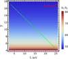 |
Fig. 2. Dependence of the ratio of the TL height to that of the disk h1/h2 on the Reynolds number γ2 = Ṁ/4πh2η2 and temperature in the TL T1 for the ratio of turbulent viscosities η2/η1 = 45. All other calculations were carried out along the diagonal line, which reflects the transition between the high/soft and low/hard states. |
The turbulent viscosity may be estimated in different ways. SS73 proposed its value as η = αρcslturb, where α is a dimensionless constant, cs is the sound speed, and lturb is a turbulent length scale, which is equal to the height h or, in addition, to the value  , where hr is the radial pressure scale hr = |p/p′| (Popham & Sunyaev 2001, PS01 hereafter). Also in radiation-pressure-dominated conditions, it may be estimated (TLM98) as η = mpnphcl/3, where mp is the proton mass, nph is the photon number density, c is the speed of light, and l is the photon mean free path. The turbulent viscosity may therefore depend on the conditions in the flow and its geometry. We avoided further reduction and took several values of the ratio of turbulent viscosities η2/η1 in order that the resulting TL lengths L be near the observable ones and also in order that γ2 corresponds to the α−1 parameter from the SS73 model.
We calculated Eqs. (10), (18), and (19) with the parameters described above for three different values of the ratio η2/η1: 30, 45, and 60. When this value is increased, there is no significant change, whereas at values far below 30, the length of the TL becomes absurdly large.
As can be seen from Fig. 3, the TL length decreases with increasing γ2. At extremely low accretion rates, the length of the TL considerably exceeds the radius of the CO, and as the accretion rate increases, the length of the TL can drop to some tenths of this radius. The motion of a gas element is a superposition of rotation with an angular velocity ω as it falls onto the CO with a velocity u, that is, it is a spiral motion. A smaller radial gas flow (i.e., smaller Ṁ and γ2) increases the distance between the coils of such a spiral, thereby making it larger. Therefore, with a fixed viscosity responsible for decreasing the angular momentum, an increase in the mass-accretion rate leads to a decrease in the TL length.
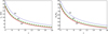 |
Fig. 3. Dependence of the TL length L (left) and the ratio (right) of the TL height to disk height h1/h2 on the Reynolds number γ2 = Ṁ/4πh2η2 for different ratios of turbulent viscosities η2/η1: 60 (solid line), 45 (dashed), and 30 (dotted). |
The behavior of the TL height h1 is similar: it is about 80 times the height of the disk at a low accretion rate and drops to about 45 times this height when the accretion rate increases (see Fig. 3). Thus, the height of the TL of a NS can be up to 1000 km in the low/hard state and half that in the high/soft state. This result can be explained easily in the frame of our model. Importantly, an increase in the mass-accretion rate at a fixed density ρ2 implies an increase in radial velocity. In this way, more matter flows through a certain area per unit of time, making the TL smaller.
7. Conclusion
We solve the problem of the transition layer (TL) geometry near a CO. We assume the CO to be weakly magnetized, and therefore only study the hydrodynamical properties of such configurations. We derived the generalized Rankine–Hugoniot relation, taking into account the different heights of the accretion disk and the TL, and the heterogeneous distributions along them. We then solved the equations of continuity and force balance in the ϕ direction and show that this latter ought to have three boundary conditions. In order to satisfy them, a TL must have certain geometric characteristics.
As a CO, we consider a NS, setting the gas parameters on both sides of the shock wave according to observations (see ST09). We then calculated the length and height of the TL. We suggest that turbulent viscosity is constant on each side of the shock, the values of which we chose such that the Reynolds number γ2 corresponds to the α−1 parameter from the SS73 model. As can be seen from Fig. 3, both the TL length and height decrease with increasing γ2. Therefore, we may conclude that:
-
We clarify the nature of the region where X-ray spectra are formed.
-
When the source evolves to a softer state, the Compton corona region becomes more compact (see Fig. 3 and also ST06, ST09). We should emphasize that the integrated power Px of the resulting power density spectra rapidly declines toward soft states (TSA07).
-
We should point out that the ratio of the TL height to the disk height h1/h2 is quite strongly dependent on the Reynolds number.
-
The calculations are carried out for a NS, although the same behavior should be expected for other types of CO (a WD or a BH).
According to the presented calculations and observed manifestations (ST06, ST09), the TL height h1 sufficiently exceeds the disk height h2. Therefore, as also noted in PS01, one-dimensional constant-height models need to be improved to correctly describe the TL.
References
- Abramowicz, M. A., & Fragile, P. C. 2013, Liv. Rev. Relat., 16, 1 [Google Scholar]
- Ajay, A., Rajesh, S. R., & Singh, N. K. 2022, ArXiv e-prints [arXiv:2210.04997] [Google Scholar]
- Chakrabarti, S. K. 1989, ApJ, 337, L89 [CrossRef] [Google Scholar]
- Chakrabarti, S., & Titarchuk, L. G. 1995, ApJ, 455, 623 [NASA ADS] [CrossRef] [Google Scholar]
- Das, P., Porth, O., & Watts, A. L. 2022, MNRAS, 515, 3144 [NASA ADS] [CrossRef] [Google Scholar]
- Farinelli, R., & Titarchuk, L. 2011, A&A, 525, A102 [NASA ADS] [CrossRef] [EDP Sciences] [Google Scholar]
- Hōshi, R. 1977, Progr. Theoret. Phys., 58, 1191 [CrossRef] [Google Scholar]
- Lančová, D., Abarca, D., Kluźniak, W., et al. 2019, ApJ, 884, L37 [CrossRef] [Google Scholar]
- Liu, B. F., & Qiao, E. 2022, Science, 25, 103544 [NASA ADS] [Google Scholar]
- Lugovskii, A. Y., & Chechetkin, V. M. 2012, Astron. Rep., 56, 96 [NASA ADS] [CrossRef] [Google Scholar]
- Matsumoto, R., Kato, S., Fukue, J., & Okazaki, A. T. 1984, PASJ, 36, 71 [NASA ADS] [Google Scholar]
- Mishra, B., Kluźniak, W., & Fragile, P. C. 2020, MNRAS, 497, 1066 [NASA ADS] [CrossRef] [Google Scholar]
- Popham, R., & Sunyaev, R. 2001, ApJ, 547, 355 [NASA ADS] [CrossRef] [Google Scholar]
- Romanova, M. M., Koldoba, A. V., Ustyugova, G. V., et al. 2021, MNRAS, 506, 372 [NASA ADS] [CrossRef] [Google Scholar]
- Seifina, E., & Titarchuk, L. 2010, ApJ, 722, 586 [NASA ADS] [CrossRef] [Google Scholar]
- Shakura, N. I., & Sunyaev, R. A. 1973, A&A, 24, 337 [NASA ADS] [Google Scholar]
- Shaposhnikov, N., & Titarchuk, L. 2009, ApJ, 699, 453 [NASA ADS] [CrossRef] [Google Scholar]
- Strohmayer, T. E., Zhang, W., Swank, J. H., et al. 1996, ApJ, 469, L9 [Google Scholar]
- Suková, P., Charzyński, S., & Janiuk, A. 2017, MNRAS, 472, 4327 [CrossRef] [Google Scholar]
- Sunyaev, R. A., & Titarchuk, L. G. 1980, A&A, 86, 121 [NASA ADS] [Google Scholar]
- Titarchuk, L., Lapidus, I., & Muslimov, A. 1998, ApJ, 499, 315 [NASA ADS] [CrossRef] [Google Scholar]
- Titarchuk, L., Shaposhnikov, N., & Arefiev, V. 2007, ApJ, 660, 556 [NASA ADS] [CrossRef] [Google Scholar]
- van der Klis, M., Swank, J. H., Zhang, W., et al. 1996, ApJ, 469, L1 [NASA ADS] [CrossRef] [Google Scholar]
- Zhang, W., Lapidus, I., White, N. E., & Titarchuk, L. 1996, ApJ, 473, L135 [CrossRef] [Google Scholar]
All Figures
|
Fig. 1. Schematic representation of the considered model. |
| In the text | |
|
Fig. 2. Dependence of the ratio of the TL height to that of the disk h1/h2 on the Reynolds number γ2 = Ṁ/4πh2η2 and temperature in the TL T1 for the ratio of turbulent viscosities η2/η1 = 45. All other calculations were carried out along the diagonal line, which reflects the transition between the high/soft and low/hard states. |
| In the text | |
|
Fig. 3. Dependence of the TL length L (left) and the ratio (right) of the TL height to disk height h1/h2 on the Reynolds number γ2 = Ṁ/4πh2η2 for different ratios of turbulent viscosities η2/η1: 60 (solid line), 45 (dashed), and 30 (dotted). |
| In the text | |
Current usage metrics show cumulative count of Article Views (full-text article views including HTML views, PDF and ePub downloads, according to the available data) and Abstracts Views on Vision4Press platform.
Data correspond to usage on the plateform after 2015. The current usage metrics is available 48-96 hours after online publication and is updated daily on week days.
Initial download of the metrics may take a while.