| Issue |
A&A
Volume 668, December 2022
|
|
|---|---|---|
| Article Number | A5 | |
| Number of page(s) | 13 | |
| Section | Extragalactic astronomy | |
| DOI | https://doi.org/10.1051/0004-6361/202244231 | |
| Published online | 28 November 2022 | |
Calibration-based abundances in the interstellar gas of galaxies from slit and IFU spectra
1
Institute of Theoretical Physics and Astronomy, Vilnius University, Sauletekio av. 3, 10257 Vilnius, Lithuania
e-mail: This email address is being protected from spambots. You need JavaScript enabled to view it.
2
Main Astronomical Observatory, National Academy of Sciences of Ukraine, 27 Akademika Zabolotnoho St, 03680 Kiev, Ukraine
3
Departamento de Física de la Tierra y Astrofísica, Universidad Complutense de Madrid, 28040 Madrid, Spain
4
Instituto de Física de Partículas y del Cosmos IPARCOS, Fac. de Ciencias Físicas, Univ. Complutense de Madrid, 28040 Madrid, Spain
5
Instituto de Astrofísica de Andalucía, CSIC, Apdo 3004, 18080 Granada, Spain
6
Département de Physique, de Génie Physique et d’Optique, Université Laval, et Centre de Recherche en Astrophysique du Québec (CRAQ), Québec, QC G1V 0A6, Canada
7
Faculty of Physics, Ludwig-Maximilians-Universität, Scheinerstr. 1, 81679 Munich, Germany
8
Universidade do Vale do Paraíba, Av. Shishima Hifumi, 2911, 12244-000 São José dos Campos, SP, Brazil
Received:
9
June
2022
Accepted:
27
September
2022
Abstract
In this work, we make use of available integral field unit (IFU) spectroscopy and slit spectra of several nearby galaxies. The pre-existing empirical R and S calibrations for abundance determinations are constructed using a sample of H II regions with high-quality slit spectra. In this paper, we test the applicability of those calibrations to the IFU spectra. We estimate the calibration-based abundances obtained using both the IFU and the slit spectroscopy for eight nearby galaxies. The median values of the slit and IFU spectra-based abundances in bins of 0.1 in fractional radius Rg (normalised to the optical radius R25) of a galaxy are determined and compared. We find that the IFU and the slit spectra-based abundances obtained through the R calibration are close to each other; the mean value of the differences of abundances is 0.005 dex, and the scatter in the differences is 0.037 dex for 38 datapoints. The S calibration can produce systematically underestimated values of the IFU spectra-based abundances at high metallicities (12 + log(O/H) ≳8.55); the mean value of the differences is −0.059 dex for 21 datapoints, while at lower metallicities the mean value of the differences is −0.018 dex and the scatter is 0.045 dex for 36 data points. This provides evidence that the R calibration produces more consistent abundance estimations between the slit and the IFU spectra than the S calibration. We find that the same calibration can produce close estimations of the abundances using IFU spectra obtained with different spatial resolution and different spatial samplings. This is in line with the recent finding that the contribution of the diffuse ionised gas to the large-aperture spectra of H II regions has a secondary effect.
Key words: ISM: abundances / H II regions / Galaxy: abundances
© L. S. Pilyugin et al. 2022
 Open Access article, published by EDP Sciences, under the terms of the Creative Commons Attribution License (https://creativecommons.org/licenses/by/4.0), which permits unrestricted use, distribution, and reproduction in any medium, provided the original work is properly cited.
This article is published in open access under the Subscribe-to-Open model. This email address is being protected from spambots. You need JavaScript enabled to view it. to support open access publication.
1. Introduction
Investigating the relations between gas-phase abundances and other characteristics of galaxies is very important for our understanding of the (chemical) evolution of galaxies. In addition to the obtained relations being affected by the absolute abundance values (i.e. metallicity scale), which depends on the adopted method for the abundance determinations, a mandatory condition in constructing such relations is for the abundances of all the galaxies to be on a unique metallicity scale. This implies that the abundances should be determined through a single method or through methods that produce abundances on the same metallicity scale. If abundances obtained using a given approach depend on the method of spectral measurement (e.g., on a part of the H II region measured) then the emission line spectra of H II regions in galaxies should be measured in a similar way.
The emission line spectra of the H II regions of galaxies available at present are measured in different ways. The long-slit spectra of the H II regions of many galaxies have been obtained in numerous investigations (e.g., see compilations in Pilyugin et al. 2004, 2014; Zurita et al. 2021). Strictly speaking, the slit spectra are not uniform in the sense that the physical fraction of the H II region within the slit can significantly vary for different reasons: (i) because of variations in slit widths in different works, (ii) because of variations in the angular sizes of the H II regions (due to variations in the physical sizes of H II regions and/or distances to galaxies), and (iii) because the slit can cross different parts (centre or periphery) of the H II regions. One can proceed by assuming (at least as a first-order approximation) that the variations in the different parts of the H II regions measured in the slit spectroscopy are random.
The integral field unit (IFU) spectroscopy measurements of the galaxy NGC 628 were carried out within the PPAK Integral Field Spectroscopy Nearby Galaxies Survey, PINGS (Sánchez et al. 2011; Rosales-Ortega et al. 2011). The 382 fibre bundle has a hexagonal field of view (FoV) of 74 arcsec × 64 arcsec. Each fibre projects to 2 7 in diameter on the sky, and the fibre-to-fibre distance is 3
 2, which yields a total filling factor of 0.6. A dithering scheme with three pointings is used to cover the complete FoV of the bundle. The spatial resolution of full width at half maximum (FWHM) is ∼2.5 arcsec. Rosales-Ortega et al. (2011) generated a catalogue of H II regions in NGC 628, and extracted the spectra of the detected H II regions. The angular size of a nearby galaxy usually exceeds the diameter of the FoV of the spectrograph. Therefore, a number of pointings are observed to form a mosaic; for example, Sánchez et al. (2011) obtained 34 pointings for NGC 628.
IFU spectroscopy measurements of a sample of galaxies on the nearby Universe were carried out in the same way (and using the same instrument as in PINGS) within the Calar Alto Legacy Integral Field Area (CALIFA) survey (Sánchez et al. 2012, 2016; García-Benito et al. 2015). Those observations have been used to construct a grid of spectra with a spatial sampling of 1″ and/or to detect H II regions and extract their spectra. The most recent version of the catalogue of H II regions includes 924 galaxies1 (Espinosa-Ponce et al. 2020).
The fibre spectra were measured in many galaxies within the Sloan Digital Sky Survey (SDSS, York et al. 2000). The SDSS spectra are obtained through 3-arcsec diameter fibres. In the framework of the SDSS IV programme, IFU spectroscopy for around 10 000 galaxies was carried out within the Mapping Nearby Galaxies at Apache Point Observatory (MaNGA) survey (Bundy et al. 2015). The diameters of the FoVs vary from 12″ (19 fibres) to 32″ (127 fibres). The final spatial sampling is 0 5/pixel, and the point spread function (PSF) of the MaNGA measurements is estimated to have a FWHM of 2.5 arcsec or 5 pixels (Bundy et al. 2015; Belfiore et al. 2017). The wavelength interval covers from 3600 to 10 300 Å with a spectral resolution of R ∼ 2000.
A sample of nearby spiral galaxies (within ∼20 Mpc) were measured within the PHANGS (Physics at High Angular Resolution in Nearby Galaxies) programme, using the Very Large Telescope/Multi Unit Spectroscopic Explorer (VLT/MUSE) to mosaic the central disc of galaxies with optical IFU observations within a 1 0–1′0 field of view with 0
 2 pixels and a typical spectral resolution of ∼2.5 Å over the wavelength range covering 4800–9300 Å (Kreckel et al. 2019). The angular resolution between galaxies varies from 0
 5 to 1
 0.
0.
An integral field spectroscopic survey of a sample of 30 nearby spiral galaxies was carried out with the Mitchell Spectrograph (formerly called VIRUS-P) IFU on the 2.7 metre telescope at McDonald Observatory within the framework of the VIRUS-P Exploration of Nearby Galaxies (VENGA) survey (Blanc et al. 2013; Kaplan et al. 2016). The Mitchell Spectrograph has a large FOV (1 7 × 1
7 × 1 7). Each fibre is 4
 2 in diameter, and the spatial resolution is 5.6 arcsec (FWHM). Each galaxy was observed with both a blue (3600–5800 Å) and a red (4600–6800 Å) setup to obtain a wide wavelength coverage. The spectral resolution is R ∼ 1000 at 5000 Å.
Using the same instrument, the IFU spectroscopy of a sample of galaxies is carried out within the ongoing Metal-THINGS survey (Lara-López et al. 2021; Lara-López 2022). This sample of galaxies is based on The H I Nearby Galaxy Survey (THINGS, Walter et al. 2008), which observed 34 nearby galaxies with the Very Large Array (VLA), providing high spatial and spectral resolution H I data. Some galaxies were observed with both a blue and a red setup, and the red spectra were observed for all galaxies.
It is widely accepted that the direct Te method produces reliable estimations of the abundances in the H II region. The auroral lines necessary for the application of the direct Te method for the abundance determinations are measured in the long-slit spectra of H II regions. The number of spectra of H II regions with detected auroral lines is steadily growing. Nevertheless, using the different variants of the strong-line method (calibrations) is the most commonly used approach to determining chemical abundances in the interstellar gas of galaxies. The H II regions with abundances determined through the direct method and the strong emission line fluxes measured in their spectra are used as the calibrating data points in the construction of the empirical calibrations (e.g., Pilyugin 2000, 2001b; Pettini & Pagel 2004; Pilyugin & Thuan 2005; Pilyugin & Mattsson 2011; Marino et al. 2013; Pilyugin & Grebel 2016; Curti et al. 2017). As those empirical calibrations are based on the slit spectra then the applicability of those calibrations for the abundance determinations using the IFU spectra is questionable.
Indeed, the spatial resolution and angular size of the native spatial sample (fibre or spaxel) can significantly exceed the angular size of the H II regions. If this is the case then the diffuse ionised gas (DIG) outside H II regions can contribute to the fibre (spaxel) spectrum as well to the extracted spectrum of the H II region. However, Mannucci et al. (2021) found that the difference between the spectra of local H II regions and those of the more distant galaxies is not due to contamination from the DIG but due to the smaller angular size of the slit with respect to the projected size of the H II regions; the DIG therefore has a secondary effect. Indeed, H II regions are stratified in the sense that higher ionisation species dominate the inner regions of nebulae while lower ionisation species are more abundant in the outer parts (see Fig. 1 in Mannucci et al. 2021 or Fig. 3 in Pérez-Montero et al. 2014). Therefore, differences can be seen between the spectra from small apertures and the spectra from larger apertures, even when both are obtained inside the H II regions.
The goal of the present work is to examine the compatibility or disagreement between the calibration-based abundances obtained using the slit spectra of H II regions and the IFU spectra of spatial samplings (fibres) or extracted IFU spectra of H II regions. The three-dimensional R calibration (O/H)R = f(R2, N2, R3/R2) and S calibration (O/H)S = f(N2, S2, R3/S2) from Pilyugin & Grebel (2016) are considered. There is no one-to-one correspondence between positions and apertures of the slit and IFU sampling. We determine the median value for abundances in bins of 0.1 in R/R25 and the scatter of each bin for both the slit and the IFU spectra-based abundances. The use of the median value in bins (the abundances at a given galactocentric distance) provides a possibility to compare the slit and IFU spectra-based abundances.
Throughout the paper, we use the following standard notations for the line intensities: R2 = I[O II]λ3727 + λ3729/IHβ, N2 = I[N II]λ6548 + λ6584/IHβ, S2 = I[S II]λ6717 + λ6731/IHβ, R3 = I[O III]λ4959 + λ5007/IHβ. We also use the standard notation for electron temperature te = 10−4Te. The galactocentric distance of the H II region or spatial sampling is given as a fractional radius Rg normalised to the optical radius R25 of a galaxy, Rg = R/R25.
2. Oxygen abundances in galaxies based on spectral measurements of different types
2.1. NGC 5457: Comparison between (O/H)Te, (O/H)R, and (O/H)S abundances based on the slit spectra
The giant nearby galaxy NGC 5457 (M 101, the Pinwheel) is a prototype of the Sc spiral galaxies (morphological type code T = 5.9 ± 0.3). NGC 5457 is a face-on galaxy, its inclination angle is i = 18°, and the position angle of the major axis PA = 37° (Kamphuis 1993). The optical radius of NGC 5457 is R25 = 14.42 arcmin (de Vaucouleurs et al. 1991).
There are 79 independent distance measurements for NGC 5457 after the year 2000 including those using Cepheids and the tip of the red giant branch (TRGB; Lomelí-Núñez et al. 2022). The obtained distances are within the range ∼6 to ∼9 Mpc. Here, we adopt the distance to NGC 5457 d = 6.85. Each characteristic of NGC 5457 is rescaled if necessary to the distance adopted here. The optical radius of NGC 5457 is R25 = 28.73 kpc with the adopted distance.
The oxygen abundance distribution across the disc of NGC 5457 is considered in a number of investigations (Kennicutt & Garnett 1996; Kennicutt et al. 2003; Pilyugin 2001a; Croxall et al. 2016; Esteban & Bresolin 2020, and references therein). As the auroral lines were measured in the spectra of a number of its H II regions and consequently the abundances in those H II regions can be derived through the direct Te method, NGC 5457 has been used to test the validity of the calibrations, that is, in some sense NGC 5457 can been considered as a ‘Rosetta stone’ (Pilyugin & Grebel 2016). Recent measurements of H II region spectra (including the auroral lines) in NGC 5457 were published by Croxall et al. (2016) and Esteban & Bresolin (2020). This provides an additional possibility to compare the abundances produced by the empirical calibrations with the direct abundances. It should be noted that the measurements from Croxall et al. (2016) and Esteban & Bresolin (2020) were not used in constructing the R and S calibrations, but the spectra of H II regions of NGC 5457 with detectable auroral lines from other publications were used.
It is believed that the Te method, based on the measurements of temperature-sensitive line ratios, should give accurate oxygen abundances. However, in practice, Te-based oxygen abundances in the same H II region derived in different works can differ for two reasons. First, there may be errors in the line-intensity measurements. Second, the Te-based oxygen abundances depend on the realisation of the Te method, that is, the derived abundances depend on the relations used to convert the values of the line fluxes to the electron temperatures and to the ion abundances. The determined abundances also depend on the adopted relationship between the electron temperature in the low-ionisation zones and that in the high-ionisation zones of nebula. The differences between the oxygen abundances at a given H II region produced by different realisations of the Te method can be appreciable (Yates et al. 2020; Cameron et al. 2021). For example, Esteban et al. (2017) found an oxygen abundance of 12 + log(O/H)Te = 8.14 ± 0.05 in the Galactic H II region Sh 2-83, while Arellano-Córdova et al. (2020) found 12 + log(O/H)Te = 8.28 ± 0.08 in the same H II region using the same spectroscopic measurements. Berg et al. (2015) detected the auroral lines in 45 H II regions in the nearby galaxy NGC 628. These authors determined the Te-based abundances in those H II regions and estimate the radial abundance gradient. They found the central (intersect) oxygen abundance 12 + log(O/H)0 = 8.83 ± 0.07 in the NGC 628. However, in their recent paper, Berg et al. (2020) recalculate ionic and total Te-based abundances in those H II regions and determine the central (intersect) oxygen abundance 12 + log(O/H)0 = 8.71 ± 0.06 for the same galaxy.
The calibration-based abundances in H II regions are determined here through the R and S calibrations from Pilyugin & Grebel (2016). The Te-based oxygen abundances in H II regions used as the calibrating data points in the construction of those calibrations are derived using the Te-method equations reported in Pilyugin et al. (2012). In order that the calibration-based and the Te-based abundances correspond to a unique abundance scale, the Te-based oxygen abundances for the H II regions in NGC 5457 are determined here using the Te-method equations from Pilyugin et al. (2012). It should be emphasised that we do not pretend that the Te-based abundances in NGC 5457 recomputed here are more accurate than the original abundances in the cited papers. We only take care that all the abundances used here correspond to the same metallicity scale. If the measurements of two auroral lines ([O III]λ4363 and [N II]λ5755 are available for the H II region then two values of the electron temperature (t3,O and t2,N) can be derived and, consequently, two independent values of the oxygen abundance ((O/H)t3,O and (O/H)t2,N) can be estimated. If the electron temperature in the low-ionisation part of the nebula t2 = t2,N is measured then the electron temperature in the high-ionisation part of the nebula t3 = t3,O is obtained using the relationship between electron temperatures in the nebula, and vice versa.
The upper panel of Fig. 1 shows the oxygen abundances estimated through the R and S calibration from Pilyugin & Grebel (2016) as a function of radius for the compilation of the slit spectra of H II regions in NGC 5457 (measurements from Croxall et al. 2016 and Esteban & Bresolin 2020 are added to the compilation in Pilyugin & Grebel 2016). Panel (b) of Fig. 1 shows the Te-based oxygen abundances of NGC 5457 H II regions from Croxall et al. (2016). Panel (c) of Fig. 1 shows the oxygen abundances of NGC 5457 H II regions from Esteban & Bresolin (2020).
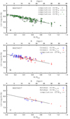 |
Fig. 1. Radial oxygen abundance distribution in NGC 5457. Panel a: calibration-based oxygen abundances for the compilation of the slit spectra of H II regions. The grey circles denote the (O/H)R abundances for individual measurements and the black solid line is the best linear fit to those data. The green plus symbols are the (O/H)S abundances for individual measurements and the dashed line is the best linear fit to those data. Panel b:Te-based oxygen abundances with measured electron temperatures t2, N (circles) and t3,O (plus signs) in H II regions from Croxall et al. (2016). The solid line is the (O/H)R–R relation from panel (a). Panel c: same as panel (b) but for the sample of H II regions from Esteban & Bresolin (2020). |
Inspection of Fig. 1 suggests that the radial abundance gradients traced by the Te-based abundances are in satisfactory agreement with those traced by the R and S calibration-based abundances determined from the slit spectra. Therefore, the slit spectra-based abundances determined through the R and S calibrations can be used as the reference abundances.
2.2. NGC 628: Comparison between abundances based on slit and IFU spectra
2.2.1. Slit-spectra-based abundances in NGC 628
The nearby galaxy NGC 628 (M 74, the Phantom Galaxy) is an isolated Sc spiral galaxy (morphological type code T = 5.2 ± 0.5) that is seen face-on, with an inclination angle of i = 6° and a position angle of the major axis PA = 25° (Kamphuis & Briggs 1992). The optical radius of this galaxy is R25 = 5.24 arcmin (de Vaucouleurs et al. 1991). The H I disc extends out to more than three times the optical radius (Kamphuis & Briggs 1992). There are recent distance estimations for NGC 628 made using the TRGB method based on the Hubble Space Telescope measurements. Jang & Lee (2014) find the distance to NGC 628 to be 10.19 ± 0.14 (random) ±0.56 (systematic) Mpc. McQuinn et al. (2017) measured the distance to M74 to be 9.77 ± 0.17 (statistical uncertainty) ±0.32 (systematic uncertainty) Mpc. Sabbi et al. (2018) determined the distances for the central pointing (d = 8.6 ± 0.9 Mpc) and for the outer field (d = 8.8 ± 0.7 Mpc). Here, we adopt the distance to NGC 628 used in our previous paper (d = 9.91 Mpc; Pilyugin et al. 2014) which is close to the values obtained by Jang & Lee (2014) and McQuinn et al. (2017). The optical radius of NGC 628 is R25 = 15.09 kpc with the adopted distance.
The slit spectra of the H II regions in the NGC 628 were measured in a number of early works (McCall et al. 1985; Ferguson et al. 1998; van Zee et al. 1998; Bresolin et al. 1999), and the slit spectroscopy of H II regions in NGC 628 were carried out within the framework of the CHemical Abundances Of Spirals (CHAOS) project (Berg et al. 2015).
The squares in panel (a) of Fig. 2 show the oxygen abundances estimated through the R calibration in individual H II regions and circles show the S calibration-based abundances. The median values of the (O/H)R and the (O/H)S together in bins of 0.1 in R/R25 are denoted by crosses, the bar marks the scatter in each bin. Panel (b) of Fig. 2 shows the comparison between median values for the (O/H)S (circles), (O/H)R (squares), and (O/H)R and (O/H)S together (crosses). The median values for different abundances are obtained for the same bin, but the positions of symbols (circles and squares) are slightly shifted along the x-axis for clarity. Inspection of panel (b) of Fig. 2 shows that the differences between the median value for (O/H)S (or (O/H)R) abundances and the median value for the (O/H)S and (O/H)R abundances together is less than the uncertainties of median values. This justifies the use of the median value for the (O/H)S and the (O/HR) abundances together instead of the median values for the (O/H)S or the (O/H)R abundances separately to specify the abundances in bins in the case of the slit-spectra-based abundances. The advantages of such an approach are as follows. First, in this case, the IFU spectra-based (O/H)S and (O/H)R abundances are compared with the same reference (slit spectra-based) abundances. Second, the slit-spectra measurements for a galaxy are usually few in number (see below); therefore, the use of (O/H)S and (O/H)R abundances together provides a possibility to estimate the median values in a larger number of bins than for the (O/H)S or the (O/H)R abundances separately. Therefore, in the case of the slit-spectra-based abundances, we estimate and use the median value in the bin for the (O/H)S and the (O/HR) abundances together and denote those median values (O/H)SLIT.
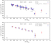 |
Fig. 2. Radial distribution of the slit-spectra-based oxygen abundances in NGC 628. Panel a: squares denote the abundances estimated through the R calibration for individual measurements, and circles are the S calibration-based abundances. The crosses mark the median value for (O/H)R and (O/H)S together in bins of 0.1 in R/R25 and the scatter of each bin. Panel b: median value for the (O/H)S (circles), (O/H)R (squares), and (O/H)R and (O/H)S together (crosses). The median values for different abundances are obtained for the same bin, but the positions of symbols (circles and squares) are slightly shifted along the x-axis for clarity. |
2.2.2. IFU spectra-based abundances in NGC 628
Rosales-Ortega et al. (2011) identified H II regions and extracted their spectra from the IFU measurements. These authors generated the H II regions catalogue for NGC 628 (PINGS catalogue). The oxygen abundances in those H II were obtained via the R calibration and are denoted by grey circles in panel (a1) of Fig. 3. Panel (a2) of Fig. 3 shows the oxygen abundances in those H II regions estimated through the S calibration. Espinosa-Ponce et al. (2020) also constructed a catalogue of H II regions in the NGC 628 using IFU observations (CALIFA catalogue). The oxygen abundance in H II regions of the CALIFA catalogue obtained through the R calibration are shown in panel (b1) of Fig. 3. Panel (b2) of Fig. 3 shows the oxygen abundances in those H II regions estimated through the S calibration. The IFU spectroscopy of the central part of NGC 628 was carried out within the framework of the PHANGS programme using the Very Large Telescope (Kreckel et al. 2019). The catalogue of the H II regions in NGC 628 was created based on those measurements. Unfortunately, only the red spectra over the wavelength range covering 4800–9300 Å were obtained. As the line [O II]λλ3727,3729 is not measured, the R calibration cannot be applied to those H II regions. Panel (c2) of Fig. 3 shows the oxygen abundances in individual H II regions estimated through the S calibration. The IFU (fibre) spectroscopy of NGC 628 was performed within the framework of the VENGA survey (Blanc et al. 2013; Kaplan et al. 2016). The oxygen abundances in the individual fibres obtained through the R calibration are denoted by grey circles in panel (d1) of Fig. 3. The grey circles in panel (d2) of Fig. 3 are the oxygen abundances in the fibres estimated through the S calibration. We compare the abundances in NGC 628 obtained from IFU spectra from different surveys to each other and to the slit-spectra-based abundances in Fig. 4.
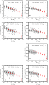 |
Fig. 3. Radial distributions of the oxygen abundances in NGC 628. Panels of columns 1–2: radial distributions of abundances estimated through the R calibration (Col. 1) and S calibration (Col. 2). Panels of rows a–d: abundances based on the IFU measurements from PINGS (row a), from CALIFA survey (row b), from PHANGS survey (row c), and from VENGA survey (row d). The grey points denote the abundances for the individual H II regions (panels of rows a, b, c) or individual spatial samplings (panels of row d), and the dark circles mark the median value in bins of 0.1 in R/R25 and the scatter of each bin. The red crosses in each panel designate the median values for the slit-spectra-based abundances (O/H)R and (O/H)S together) and come from Fig. 2. |
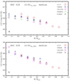 |
Fig. 4. Median values of oxygen abundances in bins of NGC 628. Panel a: median values of (O/H)S abundances based on the IFU measurements from PINGS (plus symbols), from CALIFA survey (squares), from PHANGS survey (crosses), and from VENGA survey (triangles). The median values of the abundances based on the slit measurements (circles) are obtained for the (O/H)S and (O/H)R abundances together. Panel b: same as panel (a) but for the (O/H)R abundances. |
Easeman et al. (2022) find that central dips in the metallicity profiles within galaxies can be observed using spatially resolved IFU data. It is not clear whether the dips are real or are an artefact introduced by the strong line diagnostics used to determine the metallicity. The radial changes in the (O/H)S abundances based on the PINGS and the CALIFA IFUs measurements are not perfectly monotonic; see panels (a2) and (b2) in Fig. 3. However, it is not clear whether the deviation from the monotonoc trend is caused by the decrease in the central metallicity (at R/R25 ≲ 0.2) or by the enhancement of the metallicity in the only bin, at R/R25 = 0.2–0.3. If this bin is ignored then the metallicity profile becomes monotonic. Moreover, the radial changes of the (O/H)S abundances based on the PHANGS and VENGA IFU measurements are monotonic; see panels (c2) and (d2) in Fig. 3. We therefore consider the central dip in the metallicity profile within the NGC 628 to be unlikely.
From inspection of the panels of Cols. 1 and 2 in Figs. 3 and 4 we find that the (O/H)R abundances based on the IFU spectra of H II regions from PINGS and CALIFA and spectra of fibres from VENGA are in agreement with each other and with the slit-spectra-based abundances. These comparisons also show that the (O/H)S abundances based on the IFU spectra of H II regions from PINGS, CALIFA, and PHANGS and on the IFU spectra of fibres from VENGA are similar. The IFU spectra-based (O/H)S abundances are close to the slit-spectra-based abundances at large galactocentric distances but there is a difference at smaller galactocentric distances (at high metallicities) in the sense that the IFU spectra-based (O/H)S abundances are lower than the slit spectra-based abundances. As a result, the radial abundance gradient traced by the (O/H)S abundances based on the IFU spectra is flatter than that traced by abundances based on the slit spectra. Belfiore et al. (2017) find that the galaxy inclination generates a flattening on the radial abundance gradient, because flux from different galactocentric radii is summed when the galaxy is projected in the plane of the sky. The metallicity depletion at the galaxy centre depends on the PSF and galaxy inclination and can be as large as ∼0.02 dex. As NGC 628 is a face-on galaxy (with inclination i = 6°), this effect should be minor. Unfortunately, the slit spectra measurements are not available for the central region (R/R25≲ 0.2) of NGC 628 while the IFU spectra are not available for larger radii (R/R25≳ 0.65). Therefore, the comparison is only possible within the restricted interval of galactocentric distances.
Comparison between the emission line fluxes in the slit and IFU spectra in NGC 628 can clarify the origin of the difference in abundances. Figure 5 shows the radial distributions of the emission line fluxes in the slit and the IFU spectra in NGC 628. The differences between the emission line fluxes in the slit and IFU spectra result in the differences between the slit-spectra-based and the IFU spectra-based abundances.
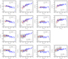 |
Fig. 5. Radial distributions of the emission line fluxes in NGC 628. Panels of columns 1–4: radial distributions of intensities of N2 line (Col. 1), R3 line (Col. 2), S2 line (Col. 3), and R2 line (Col. 4). Panels of rows a–d: IFU measurements from the surveys PINGS (row a), CALIFA (row b), PHANGS (row c), and VENGA (row d). The grey points denote the individual H II regions (panels of rows a, b, c) or individual spatial samplings (panels of row d), the red points with bars mark the median value in bins of 0.05 in R/R25 and the scatter of each bin. The blue plus symbols are individual slit measurements. As only the red spectra were measured within the PHANGS programme then the R2 line measurements are not available. |
The difference in S2 (and other lines) between different IFU measurements cannot be attributed to the difference in the spatial resolution only. If this were the case, then one would expect the S2 for a given galaxy (e.g., NGC 628) to be similar in the CALIFA and PINGS IFUs because the spatial and spectral resolutions are the same. However, there is an appreciable difference between S2 from those surveys (compare panels (a3) and (b3) in Fig. 5). One can therefore assume that the reduction in the observations (e.g., extraction of H II region spectra) and flux calibration contribute to the uncertainty in the IFU spectra and, as a consequence, produce some differences in the S2 measurements between different IFUs. However, the general behaviour of the IFU spectra-based abundances is more or less the same for different IFUs.
It may appear that (O/H)S,IFU – (O/H)SLIT is larger than (O/H)R, IFU – (O/H)SLIT (Figs. 3 and 4) because of the larger differences in the S2 flux measured between the IFU and the slit spectra. However, close examination of the available data reveals that differences in other line fluxes must also play a significant role. For example, we find that the differences in the S2 flux between PINGS and VENGA are larger than those between PINGS and CALIFA (Fig. 5), but the differences in (O/H)S between PINGS and VENGA are smaller than those between PINGS and CALIFA (Figs. 3 and 4). Moreover, at R/R25 = 0.45 to 0.50, the median values of the R2 and S2 fluxes in CALIFA and PINGS agree within ∼10% and ∼25%, respectively, and the differences between the median values of (O/H)R and (O/H)S are ∼0.01 dex and ∼0.05 dex, respectively. Whereas, at R/R25 = 0.15–0.20, the median values of the R2 and S2 fluxes in CALIFA and PINGS agree within ∼25% and ∼10%, respectively, but the differences between the median values of (O/H)R and (O/H)S are ∼0.02 dex and ∼0.03 dex, respectively. This suggests that the abundances obtained through the S calibration are affected by variations in the line fluxes more strongly than abundances obtained through the R calibration.
On the one hand, as the spatial resolutions (and sizes of the native spatial samplings) of PHANGS, CALIFA, PINGS, and VENGA observations are appreciably different, one might expect the spectra of the extracted H II regions in PHANGS to be less contaminated by the DIG than the spectra of the extracted H II regions in PINGS and CALIFA, and than the spectra of spatial samplings in VENGA. On the other hand, the shifts in the (O/H)S abundances based on the IFU spectra of PHANGS, CALIFA, PINGS, and VENGA are similar to those in the slit spectra-based abundances. Those two facts taken together are in line with the conclusion of Mannucci et al. (2021), namely that the DIG has a secondary effect.
Our investigation of the galaxy NGC 628 can be summarised as follows. (i) The oxygen abundance estimated from the IFU spectra of the extracted H II regions, or from the IFU spectra of fibres, depends weakly on the spatial resolution (and on the size of the native spatial samplings) of the IFU measurements. (ii) The R calibration applied to the IFU spectra produces more consistent abundance estimations between slit and IFU spectra than the S calibration, and the (O/H)S, IFU abundances are systematically underestimated in comparison with the slit spectra-based abundances at high metallicities. (iii) The satisfactory agreement between abundances estimated from the IFU spectra obtained with different spatial resolutions (and different sizes of the native spatial samplings) confirms the recent finding of Mannucci et al. (2021) that the DIG has a secondary effect. To confirm or reject these conclusions, we examined seven other nearby galaxies with available slit and IFU spectroscopy. The comparison between the slit and IFU spectra-based abundances for our sample of galaxies is discussed in the following section. The abundances in individual galaxies are given in Appendix A.
3. Discussion
Here, we compare and discuss the abundances based on the slit spectra and the abundances determined from the IFU spectra using the R and the S calibrations for our sample of galaxies. There are 38 bins of 0.1 in R/R25 in eight galaxies considered where the median values of both (O/H)R,IFU and (O/H)SLIT abundances are determined and 57 bins where the median values of both (O/H)S,IFU and (O/H)SLIT abundances are determined (Figs. 3, A.1–A.7).
Panel (a1) of Fig. 6 shows the abundance determined from the IFU spectra through the S calibration (median values in individual bins) as a function of the abundance obtained from the slit spectra for all eight galaxies. Panel (b1) shows the (O/H)R,IFU abundance versus the (O/H)SLIT abundances. The grey points in panel (a2) are the same data as the symbols in panel (a1) and the dark circles mark the mean value in bins of 0.05 in log(O/H)SLIT for those data points. Panel (b2) is similar to panel (a2) but compares the (O/H)R,IFU abundances. Figure 7 shows the normalised histograms of the differences between oxygen abundances (O/H)R,IFU – (O/H)SLIT for 38 data points (solid line) and between (O/H)S,IFU – (O/H)SLIT for 57 data points (dashed line). The step in the histograms is 0.02 dex.
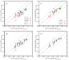 |
Fig. 6. Comparison between the abundances based on the slit spectra of H II regions and the abundances estimated from the IFU spectra of H II regions (or spatial samplings, fibres) using the R and the S calibrations. Panel a1: IFU spectra-based oxygen abundances obtained through the S calibration vs. oxygen abundances estimated from the slit spectra for our sample of galaxies (each point shows the median value in bins of 0.1 in R/R25 in individual galaxy, see Fig. 3, Figs. A.1–A.7). The abundances based on the IFU spectra from different surveys are shown by different symbols. The solid line indicates the one-to-one relation, while the dashed line shows the ±0.1 dex deviation. Panel b1: same as panel (a1) but for the IFU spectra-based abundances estimated through the R calibration. Panel a2: grey points are data from panel (a1), and the dark circles mark the mean value in bins of 0.05 in log(O/H) for those data points. Panel b2: same as panel (a2) but for the IFU spectra-based abundances estimated through the R calibration. |
Inspection of panel (a1) of Figs. 6 and 7 shows that the differences between (O/H)SLIT and (O/H)S,IFU abundances are usually less than around 0.1 dex, and the mean value of the scatter in abundance differences (O/H)S,IFU – (O/H)SLIT is 0.052 dex for the 57 data points. However, the differences are not perfectly random; the maximum of the distribution is appreciably shifted from zero; see Fig. 7. Examination of panels (a1) and (a2) of Fig. 6 shows that the (O/H)S,IFU abundances are systematically lower than the (O/H)SLIT abundances at high metallicities (12 + log(O/H) ≳ 8.55), and the mean shift of the (O/H)S, IFU abundances relative to the (O/H)SLIT abundances is −0.059 dex for 21 data points; that is, the shift of (O/H)S, IFU abundances relative to the (O/H)SLIT abundances at high metallicities exceeds the mean value of the scatter in the abundance differences.
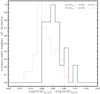 |
Fig. 7. Normalised histograms of the differences between oxygen abundances (O/H)R, IFU – (O/H)SLIT (solid line) and (O/H)S, IFU – (O/H)SLIT (dashed line). |
Inspection of panel (b1) of Figs. 6 and 7 shows that the differences between (O/H)SLIT and (O/H)R,IFU abundances are also within 0.1 dex, and the mean value of the scatter in abundance differences (O/H)R,IFU – (O/H)SLIT is 0.037 dex for the 38 data points. One can observe that the correlation between (O/H)R,IFU and (O/H)SLIT abundances is more tight than the correlation between (O/H)S, IFU and (O/H)SLIT abundances. The maximum of the abundance difference distribution is close to zero; see Fig. 7. Nevertheless, close examination of panels (b1) and (b2) of Fig. 6 shows that some correlation between the abundance difference (O/H)R,IFU – (O/H)SLIT and metallicity may exists. However, the mean shift of the (O/H)R,IFU abundances relative to the (O/H)SLIT abundances exceeds the scatter in abundance differences for one metallicity interval (12 + log(O/H) from 8.65 to 8.70) only. Therefore, it is not clear whether this weak correlation is meaningful.
Inspection of panel (a1) of Fig. 6 shows that there is agreement between the (O/H)S, IFU estimated from the IFU measurements obtained with different spatial resolutions, and panel (b1) shows that there is similar agreement for the (O/H)R,IFU abundances. This suggests that the IFU spectra-based abundances depend weakly (if any) on the spatial resolution of the IFU measurements. Indeed, there is agreement between the (O/H)S, IFU abundances estimated in NGC 4254 from the VENGA measurements (panel (b) in Fig. A.5) and from the PHANGS measurements (panel (d) in Fig. A.5) although the spatial resolution of the VENGA measurements is significantly lower than that of the PHANGS measurements. Moreover, the agreement between (O/H)S, IFU abundances estimated in NGC 628 from the PINGS and the VENGA measurements obtained with different spatial resolutions is better than the agreement between (O/H)S, IFU abundances estimated from the PINGS and the CALIFA measurements obtained with the same spatial resolution; see Fig. 4.
The comparison between the slit and the IFU spectra-based abundances for our sample of galaxies in this section confirms our above conclusions for the galaxy NGC 628. It should be emphasised that the abundances analysed here are distributed over a limited interval of metallicity, from 12 + log(O/H) ∼8.4 to ∼8.7 only (with one exception). In order to strengthen (or reject) our conclusions and derive the relationships between the IFU and slit-spectra-based abundances, abundances distributed over a larger range of metallicity are required.
4. Conclusions
Calibration-based abundances are considered in eight nearby galaxies, where both the slit spectra of H II regions and the spectra of H II regions extracted from the IFU measurements (PINGS, CALIFA, and PHANGS surveys) or the IFU spectra of spatial samplings (VENGA and Metal-THINGS surveys) are available. The pre-existing empirical R and S calibrations for abundance determinations were constructed using a sample of H II regions with high-quality slit spectra (Pilyugin & Grebel 2016). In this study, we test the applicability of those calibrations to the IFU spectra. We estimate the R and S calibration-based abundances using both the IFU and the slit spectroscopy for eight nearby galaxies. The median values of the IFU spectra-based abundances (O/H)R, IFU and (O/H)S, IFU in bins of 0.1 in fractional radius Rg (normalised to the optical radius R25) are determined for each galaxy and are compared to the median values of the slit spectra-based abundances (O/H)SLIT determined using both the (O/H)R and (O/H)S abundances together.
We find that the differences between (O/H)SLIT and (O/H)S, IFU abundances are usually less than around 0.1 dex, and that the mean value of the scatter in abundance differences (O/H)S, IFU – (O/H)SLIT is 0.052 dex for 57 data points. However, the (O/H)S, IFU abundances are systematically lower than the (O/H)SLIT abundances at high metallicities (12 + log(O/H) ≳ 8.55), and the mean shift of the (O/H)S, IFU abundances relative to the (O/H)SLIT abundances is around −0.06 dex for 21 data points. The differences between the intensities of each line (used in the abundance determinations) in the slit and the IFU spectra contribute to the differences between the abundances based on the slit and the IFU spectra. Our data indicate that the abundances estimated through the S calibration are more sensitive to variations in the line fluxes than the abundances obtained using the R calibration.
The correlation between (O/H)R, IFU and (O/H)SLIT abundances is tighter than the correlation between (O/H)S, IFU and (O/H)SLIT abundances. The mean value of the scatter in abundance differences (O/H)R, IFU – (O/H)SLIT is 0.037 dex for 38 data points. We see evidence for a weak correlation between the abundance difference (O/H)R, IFU – (O/H)SLIT and metallicity. However, the mean shift of the (O/H)R, IFU abundances relative (O/H)SLIT abundances is less than the scatter in abundance differences for all but one of the metallicity intervals of 0.05 dex. Therefore, it is not clear whether or not this weak correlation is meaningful.
We find that the same calibration can produce close estimations of the abundances using the IFU spectra (of extracted H II regions or spatial samplings) from the IFU measurements carried out with different spatial resolution and different native spatial samplings. This is in line with the finding of Mannucci et al. (2021) that the contribution of the diffuse ionised gas to the large-aperture spectra of H II regions has a secondary effect.
Acknowledgments
We are grateful to the referee for his/her constructive comments. We thank the VENGA collaboration for providing access to the data. L.S.P acknowledges support from the Research Council of Lithuania (LMTLT) (grant no. P-LU-PAR-22-7). MALL acknowledges support from the Spanish grant PID2021-123417OB-I00. SDP is grateful to the Fonds de Recherche du Québec – Nature et Technologies. JVM and SDP acknowledge financial support from the Spanish Ministerio de Economía y Competitividad under grants AYA2016-79724-C4-4-P and PID2019-107408GB-C44, from Junta de Andalucía Excellence Project P18-FR-2664, and also acknowledge support from the State Agency for Research of the Spanish MCIU through the ‘Center of Excellence Severo Ochoa’ award for the Instituto de Astrofísica de Andalucía (SEV-2017-0709). This study makes use of the results based on the Calar Alto Legacy Integral Field Area (CALIFA) survey (http://califa.caha.es/).
References
- Anand, G. S., Lee, J. C., Van Dyk, S. D., et al. 2021, MNRAS, 501, 3621 [Google Scholar]
- Arellano-Córdova, K. Z., Esteban, C., García-Rojas, J., & Méndez-Delgado, J. E. 2020, MNRAS, 496, 1051 [Google Scholar]
- Belfiore, F., Maiolino, R., Tremonti, C., et al. 2017, MNRAS, 469, 151 [Google Scholar]
- Berg, D. A., Skillman, E. D., Croxall, K. V., et al. 2015, ApJ, 806, 16 [NASA ADS] [CrossRef] [Google Scholar]
- Berg, D. A., Pogge, R. W., Skillman, E. D., et al. 2020, ApJ, 893, 96 [NASA ADS] [CrossRef] [Google Scholar]
- Blanc, G. A., Schruba, A., Evans, N. J., et al. 2013, ApJ, 764, 117 [NASA ADS] [CrossRef] [Google Scholar]
- Bresolin, F. 2019, MNRAS, 488, 3826 [NASA ADS] [Google Scholar]
- Bresolin, F., Kennicutt, R. C., & Garnett, D. R. 1999, ApJ, 510, 104 [NASA ADS] [CrossRef] [Google Scholar]
- Bresolin, F., Garnett, D. R., & Kennicutt, R. C. 2004, ApJ, 615, 228 [NASA ADS] [CrossRef] [Google Scholar]
- Bresolin, F., Schaerer, D., González Delgado, R. M., & Stasińska, G. 2005, A&A, 441, 981 [NASA ADS] [CrossRef] [EDP Sciences] [Google Scholar]
- Bundy, K., Bershady, M. A., Law, D. R., et al. 2015, ApJ, 798, 7 [Google Scholar]
- Cameron, A. J., Yuan, T., Trenti, M., Nicholls, D. C., & Kewley, L. J. 2021, MNRAS, 501, 3695 [NASA ADS] [Google Scholar]
- Colombo, D., Meidt, S. E., Schinnerer, E., et al. 2014, ApJ, 784, 4 [Google Scholar]
- Croxall, K. V., Pogge, R. W., Berg, D. A., Skillman, E. D., & Moustakas, J. 2015, ApJ, 808, 42 [NASA ADS] [CrossRef] [Google Scholar]
- Croxall, K. V., Pogge, R. W., Berg, D. A., Skillman, E. D., & Moustakas, J. 2016, ApJ, 830, 4 [NASA ADS] [CrossRef] [Google Scholar]
- Curti, M., Cresci, G., Mannucci, F., et al. 2017, MNRAS, 465, 1384 [Google Scholar]
- Davis, B. L., Berrier, J. C., Johns, L., et al. 2014, ApJ, 789, 124 [NASA ADS] [CrossRef] [Google Scholar]
- de Blok, W. J. G., Walter, F., Brinks, E., et al. 2008, AJ, 136, 2648 [NASA ADS] [CrossRef] [Google Scholar]
- de Vaucouleurs, G., de Vaucouleurs, A., Corvin, H. G., et al. 1991, Third Reference Catalog of bright Galaxies (New York: Springer Verlag (RC3)) [Google Scholar]
- Díaz, Á., Terlevich, E., Vilchez, J. M., Pagel, B. E. J., & Edmunds, M. 1991, MNRAS, 253, 245 [NASA ADS] [CrossRef] [Google Scholar]
- Díaz, Á, Terlevich, E., Castellanos, M., & Hägele, G. 2007, MNRAS, 382, 251 [CrossRef] [Google Scholar]
- Drozdovsky, I. O., & Karachentsev, I. D. 2000, A&AS, 142, 425 [NASA ADS] [CrossRef] [EDP Sciences] [Google Scholar]
- Easeman, B., Schady, P., Wuyts, S., & Yates, R. M. 2022, MNRAS, 511, 371 [NASA ADS] [CrossRef] [Google Scholar]
- Espinosa-Ponce, C., Sánchez, S. F., Morisset, C., et al. 2020, MNRAS, 494, 1622 [Google Scholar]
- Esteban, C., Fang, X., García-Rojas, J., & Toribio San Cipriano, L. 2017, MNRAS, 471, 987 [NASA ADS] [CrossRef] [Google Scholar]
- Esteban, C., Bresolin, F., García-Rojas, J., & Toribio San Cipriano, L. 2020, MNRAS, 491, 2137 [NASA ADS] [Google Scholar]
- Ferguson, A. M. N., Gallagher, J. S., & Wyse, R. F. G. 1998, AJ, 116, 673 [NASA ADS] [CrossRef] [Google Scholar]
- García-Benito, R., Díaz, A., Hägele, G. F., et al. 2010, MNRAS, 408, 2234 [CrossRef] [Google Scholar]
- García-Benito, R., Zibetti, S., Sánchez, S. F., et al. 2015, A&A, 576, A135 [Google Scholar]
- García-Gómez, C., Barberà, C., Athanassoula, E., Bosma, A., & Whyte, L. 2004, A&A, 421, 595 [NASA ADS] [CrossRef] [EDP Sciences] [Google Scholar]
- Garnett, D., Kennicutt, R. C., & Bresolin, F. 2004, ApJ, 607, L21 [NASA ADS] [CrossRef] [Google Scholar]
- Henry, R. B. C., Pagel, B. E. J., & Chincarini, G. L. 1994, MNRAS, 266, 421 [NASA ADS] [CrossRef] [Google Scholar]
- Jang, I. S., & Lee, M. G. 2014, ApJ, 792, 52 [NASA ADS] [CrossRef] [Google Scholar]
- Jarrett, T. H., Cluver, M. E., Brown, M. J. I., et al. 2019, ApJS, 245, 25 [Google Scholar]
- Kamphuis, J. J. 1993, PhD Thesis, Univ. Groningen, The Netherlands [Google Scholar]
- Kamphuis, J., & Briggs, F. 1992, A&A, 253, 335 [NASA ADS] [Google Scholar]
- Kaplan, K. F., Jogee, S., Kewley, L., et al. 2016, MNRAS, 462, 1642 [NASA ADS] [CrossRef] [Google Scholar]
- Kennicutt, R. C., & Garnett, D. R. 1996, ApJ, 456, 504 [NASA ADS] [CrossRef] [Google Scholar]
- Kennicutt, R. C., Bresolin, F., & Garnett, D. R. 2003, ApJ, 591, 801 [NASA ADS] [CrossRef] [Google Scholar]
- Kreckel, K., Ho, I.-T., Blanc, G. A., et al. 2019, ApJ, 887, 80 [NASA ADS] [CrossRef] [Google Scholar]
- Lang, P., Meidt, S., Rosolowsky, E., et al. 2020, ApJ, 897, 122 [CrossRef] [Google Scholar]
- Lara-López, M., Zinchenko, I., Pilyugin, L., et al. 2021, ApJ, 906, 42 [CrossRef] [Google Scholar]
- Lara-López, M., Pilyugin, L. S., Zaragoza-Cardiel, J., et al. 2022, A&A, in press, https://doi.org/10.1051/0004-6361/202245068 [Google Scholar]
- Leroy, A. K., Walter, F., Brinks, E., et al. 2008, AJ, 136, 2782 [Google Scholar]
- Leroy, A. K., Sandstrom, K., Lang, D., et al. 2019, ApJS, 244, 24 [NASA ADS] [CrossRef] [Google Scholar]
- Leroy, A. K., Schinnerer, E., Hughes, A., et al. 2021, ApJS, 257, 43 [NASA ADS] [CrossRef] [Google Scholar]
- Lomelí-Núñez, L., Mayya, Y. D., Rodríguez-Merino, L. H., Ovando, P. A., & Rosa-González, D. 2022, MNRAS, 509, 180 [Google Scholar]
- Mannucci, F., Belfiore, F., Curti, M., et al. 2021, MNRAS, 508, 1582 [NASA ADS] [CrossRef] [Google Scholar]
- Marino, R. A., Rosales-Ortega, F. F., Sánchez, S. F., et al. 2013, A&A, 559, A114 [NASA ADS] [CrossRef] [EDP Sciences] [Google Scholar]
- McCall, M. L., Rybski, P. M., & Shields, G. A. 1985, ApJS, 57, 1 [CrossRef] [Google Scholar]
- McQuinn, K. B. W., Skillman, E. D., Dolphin, A. E., Berg, D., & Kennicutt, R. 2017, AJ, 154, 51 [NASA ADS] [CrossRef] [Google Scholar]
- Pérez-Montero, E., Monreal-Ibero, A., Relaño, M., et al. 2014, A&A, 566, A12 [NASA ADS] [CrossRef] [EDP Sciences] [Google Scholar]
- Pettini, M., & Pagel, B. E. J. 2004, MNRAS, 348, L59 [NASA ADS] [CrossRef] [Google Scholar]
- Pilyugin, L. S. 2000, A&A, 362, 325 [NASA ADS] [Google Scholar]
- Pilyugin, L. S. 2001a, A&A, 369, 594 [NASA ADS] [CrossRef] [EDP Sciences] [Google Scholar]
- Pilyugin, L. S. 2001b, A&A, 373, 56 [NASA ADS] [CrossRef] [EDP Sciences] [Google Scholar]
- Pilyugin, L. S., & Thuan, T. X. 2005, ApJ, 631, 231 [CrossRef] [Google Scholar]
- Pilyugin, L. S., & Mattsson, L. 2011, MNRAS, 412, 1145 [NASA ADS] [Google Scholar]
- Pilyugin, L. S., & Grebel, E. K. 2016, MNRAS, 457, 3678 [NASA ADS] [CrossRef] [Google Scholar]
- Pilyugin, L. S., Vílchez, J. M., & Contini, T. 2004, A&A, 425, 849 [NASA ADS] [CrossRef] [EDP Sciences] [Google Scholar]
- Pilyugin, L. S., Grebel, E. K., & Mattsson, L. 2012, MNRAS, 424, 2316 [NASA ADS] [CrossRef] [Google Scholar]
- Pilyugin, L. S., Grebel, E. K., & Kniazev, A. Y. 2014, AJ, 147, 131 [NASA ADS] [CrossRef] [Google Scholar]
- Rosales-Ortega, F. F., Díaz, A. I., Kennicutt, R. C., & Sánchez, S. F. 2011, MNRAS, 415, 2439 [NASA ADS] [CrossRef] [Google Scholar]
- Rots, A. H., Bosma, A., van der Hulst, J. M., Athanassoula, E., & Crane, P. C. 1990, AJ, 100, 387 [NASA ADS] [CrossRef] [Google Scholar]
- Ryder, S. D. 1995, ApJ, 444, 610 [NASA ADS] [CrossRef] [Google Scholar]
- Sabbi, E., Calzetti, D., Ubeda, L., et al. 2018, ApJS, 235, 23 [Google Scholar]
- Sánchez, S. F., Rosales-Ortega, F. F., Kennicutt, R. C., et al. 2011, MNRAS, 410, 313 [CrossRef] [Google Scholar]
- Sánchez, S. F., Kennicutt, R. C., Gil de Paz, A., et al. 2012, A&A, 538, A8 [Google Scholar]
- Sánchez, S. F., García-Benito, R., Zibetti, S., et al. 2016, A&A, 594, A36 [Google Scholar]
- Schmidt, B. P., Kirshner, R. P., Eastman, R. G., et al. 1994, ApJ, 432, 42 [NASA ADS] [CrossRef] [Google Scholar]
- Shields, G. A., Skillman, E. D., & Kennicutt, R. C. 1991, ApJ, 371, 825 [NASA ADS] [CrossRef] [Google Scholar]
- Storchi-Bergmann, T., Wilson, A. S., & Baldwin, J. A. 1996, ApJ, 460, 252 [NASA ADS] [CrossRef] [Google Scholar]
- Tamburro, D., Rix, H.-W., Walter, F., et al. 2008, AJ, 136, 2872 [NASA ADS] [CrossRef] [Google Scholar]
- van den Bosch, R. C. E. 2016, ApJ, 831, 134 [NASA ADS] [CrossRef] [Google Scholar]
- van Zee, L., Salzer, J. J., Haynes, M. P., O‘Donoghue, A. A., & Balonek, T. J. 1998, AJ, 116, 2805 [CrossRef] [Google Scholar]
- Walter, F., Brinks, E., de Blok, W. J. G., et al. 2008, AJ, 136, 2563 [Google Scholar]
- Yates, R. M., Schady, P., Chen, T.-W., Schweyer, T., & Wiseman, P. 2020, A&A, 634, A107 [NASA ADS] [CrossRef] [EDP Sciences] [Google Scholar]
- York, D. G., Adelman, J., Anderson, J. E., et al. 2000, AJ, 120, 1579 [Google Scholar]
- Zurita, A., Florido, E., Bresolin, F., Pérez-Montero, E., & Pérez, I. 2021, MNRAS, 500, 2359 [Google Scholar]
Appendix A: Abundances based on slit and IFU spectra in nearby galaxies
Here we estimate the oxygen abundances based on the slit and the IFU spectra in seven nearby galaxies with available slit and IFU spectroscopy. The (O/H)R, IFU and/or (O/H)S, IFU abundances for individual IFU spectra as well as the median abundances in bins of 0.1 in fractional radius R/R25 are determined. The median values of the slit spectra-based abundances (O/H)SLIT are determined using both the (O/H)R and the (O/H)S abundances for individual H II regions together. The medial value is determined if the number of points in the bin is larger than three. The abundances in each galaxy are shown below; see Fig. A.1 – A.7. The data for that sample of galaxies (together with the data for NGC 628) are presented in Figs. 6 and 7 and are used in our discussion in Section 3.
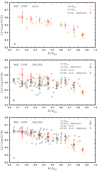 |
Fig. A.1. Radial oxygen abundance distribution in NGC 1058. Panel a: Oxygen abundances based on the slit spectra of H II regions. The squares denote the abundances estimated through the R calibration for individual measurements, the circles designate the (O/H)S abundances. The crosses mark the median values of the slit spectra-based abundances in bins of 0.1 in the fractional radius determined using both the (O/H)R and the (O/H)S abundances for individual H II regions together. The bar shows the scatter in each bin. Panel b: Grey points denote the (O/H)S, IFU abundances based on the extracted IFU (CALIFA) spectra of individual H II regions. The dark circles mark the median values in bins, and bar shows the scatter in each bin. The crosses mark the median values of the slit spectra-based abundances and come from panel (a). Panel c: Same as panel (b) but for the (O/H)R, IFU abundances. |
A.1. NGC 1058
NGC 1058 is a Sc galaxy (morphological type code T = 5.1±0.9). The inclination angle of NGC 1058 is i = 15°, the position angle of the major axis PA = 145° (García-Gómez et al. 2004). The optical radius is 1.51 arcmin (de Vaucouleurs et al. 1991). At the distance of d = 10.6 Mpc (Schmidt et al. 1994), the physical optical radius is R25 = 4.66 kpc. The stellar mass (rescaled to the adopted distance) is M⋆ = 2.51 × 10⁹ M⊙ (Leroy et al. 2019).
The slit spectra of H II regions in NGC 1058 were measured by Ferguson et al. (1998) and Bresolin (2019). Panel (a) of Fig. A.1 shows the slit spectra-based oxygen abundances. The IFU spectroscopy of NGC 1058 was carried out within the CALIFA survey. Panel (b) of Fig. A.1 shows the IFU spectra-based (O/H)S abundances in NGC 1058. The line flux measurements in the spectra of H II regions are taken from the catalogue of H II regions (cited above). Panel (c) of Fig. A.1 shows the same as panel (b) but for (O/H)R abundances.
A.2. NGC 1672
NGC 1672 is a Sb galaxy (morphological type code T = 3.3±0.6). The inclination angle of NGC 1672 is i = 43°, and the position angle of the major axis PA = 134° (Lang et al. 2020). The optical radius is 3.30 arcmin (de Vaucouleurs et al. 1991). At the distance of d = 19.40 Mpc (Anand et al. 2021), the physical optical radius is R25 = 18.64 kpc. The stellar mass is M⋆ = 5.37 × 10¹⁰ M⊙ (Leroy et al. 2021). NGC 1672 hosts a central black hole of mass logMBH = 7.08±0.90 in solar mass (Davis et al. 2014).
The slit spectra of H II regions in NGC 1672 were measured by Storchi-Bergmann et al. (1996). The slit spectra-based (O/H)R and (O/H)S abundances are shown in panel (a) of Fig. A.2. The IFU spectroscopy of NGC 1672 was carried out within the framework of the PHANGS programme (Kreckel et al. 2019). The catalogue of the H II regions in NGC 1672 was created on the base of those measurements. Unfortunately, only the red spectra over the wavelength range covering 4800-9300Å were obtained. As the line [O II]λλ3727,3729 is not measured then the R calibration cannot be applied to those H II regions. Panel (b) of Fig. A.2 shows the IFU spectra-based oxygen abundances estimated through the S calibration.
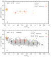 |
Fig. A.2. Radial oxygen abundance distribution in NGC 1672. Panel a: Oxygen abundances based on the slit spectra of H II regions. Panel b: Oxygen abundances based on the IFU (PHANGS) spectra of H II regions. The notations are the same as in Fig. A.1. |
A.3. NGC 2835
NGC 2835 is a Sc galaxy (morphological type code T = 5.0±0.4). The inclination angle of NGC 2835 is i = 51° (Ryder 1995), the position angle of the major axis PA = 1° (Lang et al. 2020). The optical radius is 3.30 arcmin (de Vaucouleurs et al. 1991). At the distance of d = 12.22 Mpc (Anand et al. 2021), the physical optical radius is R25 = 11.74 kpc. The stellar mass is M⋆ = 1.0 × 10¹⁰ M⊙ (Leroy et al. 2021). The mass of the central black hole in NGC 2835 is logMBH = 6.72±0.30 in solar mass (Davis et al. 2014).
The slit spectra of H II regions in NGC 2835 were measured by Ryder (1995). Panel (a) of Fig. A.3 shows the oxygen abundances in those H II regions. The IFU spectroscopy of NGC 2835 was carried out within the framework of the PHANGS programme and a catalogue of H II regions was created (Kreckel et al. 2019). Panel (b) of Fig. A.3 shows the IFU spectra-based oxygen abundances in NGC 2835.
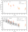 |
Fig. A.3. Radial oxygen abundance distribution in NGC 2835. Panel a: Oxygen abundances based on the slit spectra of H II regions. Panel b: Oxygen abundances based on the IFU (PHANGS) spectra of H II regions. The notations are the same as in Fig. A.1. |
A.4. NGC 2903
The nearby galaxy NGC 2903 is a Sbc spiral galaxy (morphological type code T = 4.0±0.1). Its inclination angle is i = 65° and the position angle of the major axis PA = 204° (de Blok et al. 2008). The optical radius of NGC 2903 is R25 = 5.87 arcmin (Walter et al. 2008). The distance to NGC 2903 is d = 8.9 Mpc (Drozdovsky & Karachentsev 2000), which results in the physical optical radius of R25 = 15.21 kpc. The mean value of the estimations of the stellar mass of NGC 2903 (rescaled to the adopted distance) is M⋆ = 3.33 × 10¹⁰ M⊙ (Jarrett et al. 2019; Leroy et al. 2021). NGC 2903 hosts a supermassive black hole of mass logMBH = 7.06 in solar mass (van den Bosch 2016).
The slit spectra of H II regions in the disc of NGC 2903 were measured by McCall et al. (1985), van Zee et al. (1998), Bresolin et al. (2005), and Díaz et al. (2007). Panel (a) of Fig. A.4 shows the oxygen abundances in those H II regions. The IFU (fibre) spectroscopy of NGC 2903 was performed within the framework of the VENGA survey (Blanc et al. 2013; Kaplan et al. 2016). Panel (b) of Fig. A.4 shows the IFU spectra-based (O/H)S, IFU abundances. Panel (c) of Fig. A.4 shows the same as panel (b) but for (O/H)R, IFU abundances.
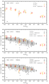 |
Fig. A.4. Radial oxygen abundance distribution in NGC 2903. Panel a: oxygen abundances based on the slit spectra of H II regions. Panel b: oxygen abundances estimated through the S calibration from the IFU (VENGA) spectra of fibres. Panel c: oxygen abundances obtained through the R calibration from the IFU (VENGA) spectra of fibres. The notations are the same as in Fig. A.1. |
A.5. NGC 4254
NGC 4254 (M 99) is a bright Sc galaxy (morphological type code T = 5.2±0.7) in the Virgo Cluster. The inclination angle of NGC 4254 is i = 34°, the position angle of the major axis PA = 68° (Lang et al. 2020). The optical radius is 2.68 arcmin (de Vaucouleurs et al. 1991). At the distance of d = 13.1 Mpc (Anand et al. 2021), the physical optical radius is R25 = 10.23 kpc. The stellar mass is M⋆ = 2.63 × 10¹⁰ M⊙ (Leroy et al. 2021).
The slit spectra of H II regions in the disc of NGC 4254 were measured by McCall et al. (1985), Shields et al. (1991), and Henry et al. (1994). Panel (a) of Fig. A.5 shows the slit spectra-based oxygen abundances. The IFU spectroscopy of NGC 4254 was carried out within the framework of the VENGA survey (Blanc et al. 2013; Kaplan et al. 2016). Panel (b) of Fig. A.5 shows the individual fibre (O/H)S, IFU abundances, and the median values in bins for those data. Panel (c) of Fig. A.5 shows the same as panel (b) but for the (O/H)R, IFU abundances. The IFU spectroscopy of NGC 4254 was also carried out within the framework of the PHANGS programme and the catalogue of H II regions was constructed (Kreckel et al. 2019). Panel (d) of Fig. A.5 shows the (O/H)S, IFU abundances based on the IFU spectra of H II regions, and the median values in bins for those data.
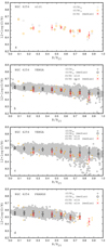 |
Fig. A.5. Radial oxygen abundance distribution in NGC 4254. Panel a: Oxygen abundances based on the slit spectra of H II regions. Panel b: Oxygen abundances estimated through the S calibration from the IFU (VENGA) spectra of fibres. Panel c: Oxygen abundances obtained through the R calibration from the IFU (VENGA) spectra of fibres. Panel d: Oxygen abundances estimated through the S calibration from the IFU (PHANGS) spectra of H II regions. The notations are the same as in Fig. A.1. |
A.6. NGC 5194
The nearby galaxy NGC 5194 (M 51a, the Whirlpool Galaxy) is a SABb spiral galaxy (morphological type code T = 4.0±0.3). The bright disc of NGC 5194 ends abruptly at about 5 arcmin radius in both the optical images and the H I. The velocity structure of the gas in NGC 5194 is extremely complicated and difficult to interpret (Rots et al. 1990). There is the misalignment of the major axes of the H I distribution and the velocity field. Therefore the geometrical parameters of NGC 5194 are rather uncertain. Tamburro et al. (2008) derive the following geometrical projection parameters of the NGC 5194 galactic disc: position angle PA = 172° and inclination i = 42°. Colombo et al. (2014) undertake a detailed kinematic study of NGC 5194 and found a position angle PA = (173 ± 3)°, and an inclination i = (22 ± 5)°. The geometrical parameters of NGC 5194 obtained by Colombo et al. (2014) are used here. We adopt the optical radius of NGC 5194 to be R25 = 5.61 arcmin (de Vaucouleurs et al. 1991). It should be noted that the value of the optical radius of R25 = 3.88 arcmin is used for NGC 5194 within The H I Nearby Galaxy Survey (THINGS) (Walter et al. 2008). There are recent distance estimations for NGC 5194 through the tip of the red giant branch (TRGB) method based on the Hubble Space Telescope measurements. Here we adopt the distance to NGC 5194 as d = 8.58 Mpc, obtained by McQuinn et al. (2017). The optical radius of NGC 5194 is R25 = 14.00 kpc with adopted distance. The stellar mass rescaled to the adopted distance is M⋆ = 4.54 × 10¹⁰ M⊙ (Leroy et al. 2008; Jarrett et al. 2019).
The slit spectra of H II regions in NGC 5194 were measured in a number of works (McCall et al. 1985; Díaz et al. 1991; Bresolin et al. 1999, 2004; Garnett et al. 2004; Croxall et al. 2015). Panel (a) of Fig. A.6 shows the slit spectra-based oxygen abundances. The IFU spectroscopy of NGC 5194 was performed within the framework of the VENGA survey (Blanc et al. 2013; Kaplan et al. 2016). Panel (b) of Fig. A.6 shows the fibre (O/H)S abundances and the median values in bins.
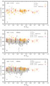 |
Fig. A.6. Radial oxygen abundance distribution in NGC 5194. Panel a: Oxygen abundances based on the slit spectra of H II regions. Panel b: Oxygen abundances estimated through the S calibration from the IFU (VENGA) spectra of fibres. Panel c: Oxygen abundances obtained through the R calibration from the IFU (VENGA) spectra of fibres. The notations are the same as in Fig. A.1. |
A.7. NGC 6946
NGC 6946 is SABc galaxy (morphological type code T = 5.9±0.3). The inclination angle of NGC 6946 is i = 33°, and the position angle of the major axis PA = 243° (de Blok et al. 2008). The optical radius is 5.74 arcmin (de Vaucouleurs et al. 1991). At the distance of d = 7.34 Mpc (Anand et al. 2021), the physical optical radius is R25 = 12.26 kpc. The stellar mass (mean value) is M⋆ = 2.85 × 10¹⁰ M⊙ (Jarrett et al. 2019; Leroy et al. 2019).
The slit spectra of H II regions in NGC 6946 were measured by McCall et al. (1985), Ferguson et al. (1998), and García-Benito et al. (2010). Panel (a) of Fig. A.7 show the slit spectra-based oxygen abundances. The IFU spectroscopy of NGC 6946 was carried out within the framework of the Metal-THINGS programme (Lara-López 2022). Only the red spectra over the wavelength range covering 4800-9300Å were obtained. Panel (b) of Fig. A.7 shows the oxygen abundances in individual fibres and the median values in bins.
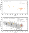 |
Fig. A.7. Radial oxygen abundance distribution in NGC 6946. Panel a: Oxygen abundances based on the slit spectra of H II regions. Panel b: Oxygen abundances estimated through the S calibration from the IFU (Metal-THINGS) spectra of fibres. The notations are the same as in Fig. A.1. |
All Figures
|
Fig. 1. Radial oxygen abundance distribution in NGC 5457. Panel a: calibration-based oxygen abundances for the compilation of the slit spectra of H II regions. The grey circles denote the (O/H)R abundances for individual measurements and the black solid line is the best linear fit to those data. The green plus symbols are the (O/H)S abundances for individual measurements and the dashed line is the best linear fit to those data. Panel b:Te-based oxygen abundances with measured electron temperatures t2, N (circles) and t3,O (plus signs) in H II regions from Croxall et al. (2016). The solid line is the (O/H)R–R relation from panel (a). Panel c: same as panel (b) but for the sample of H II regions from Esteban & Bresolin (2020). |
| In the text | |
|
Fig. 2. Radial distribution of the slit-spectra-based oxygen abundances in NGC 628. Panel a: squares denote the abundances estimated through the R calibration for individual measurements, and circles are the S calibration-based abundances. The crosses mark the median value for (O/H)R and (O/H)S together in bins of 0.1 in R/R25 and the scatter of each bin. Panel b: median value for the (O/H)S (circles), (O/H)R (squares), and (O/H)R and (O/H)S together (crosses). The median values for different abundances are obtained for the same bin, but the positions of symbols (circles and squares) are slightly shifted along the x-axis for clarity. |
| In the text | |
|
Fig. 3. Radial distributions of the oxygen abundances in NGC 628. Panels of columns 1–2: radial distributions of abundances estimated through the R calibration (Col. 1) and S calibration (Col. 2). Panels of rows a–d: abundances based on the IFU measurements from PINGS (row a), from CALIFA survey (row b), from PHANGS survey (row c), and from VENGA survey (row d). The grey points denote the abundances for the individual H II regions (panels of rows a, b, c) or individual spatial samplings (panels of row d), and the dark circles mark the median value in bins of 0.1 in R/R25 and the scatter of each bin. The red crosses in each panel designate the median values for the slit-spectra-based abundances (O/H)R and (O/H)S together) and come from Fig. 2. |
| In the text | |
|
Fig. 4. Median values of oxygen abundances in bins of NGC 628. Panel a: median values of (O/H)S abundances based on the IFU measurements from PINGS (plus symbols), from CALIFA survey (squares), from PHANGS survey (crosses), and from VENGA survey (triangles). The median values of the abundances based on the slit measurements (circles) are obtained for the (O/H)S and (O/H)R abundances together. Panel b: same as panel (a) but for the (O/H)R abundances. |
| In the text | |
|
Fig. 5. Radial distributions of the emission line fluxes in NGC 628. Panels of columns 1–4: radial distributions of intensities of N2 line (Col. 1), R3 line (Col. 2), S2 line (Col. 3), and R2 line (Col. 4). Panels of rows a–d: IFU measurements from the surveys PINGS (row a), CALIFA (row b), PHANGS (row c), and VENGA (row d). The grey points denote the individual H II regions (panels of rows a, b, c) or individual spatial samplings (panels of row d), the red points with bars mark the median value in bins of 0.05 in R/R25 and the scatter of each bin. The blue plus symbols are individual slit measurements. As only the red spectra were measured within the PHANGS programme then the R2 line measurements are not available. |
| In the text | |
|
Fig. 6. Comparison between the abundances based on the slit spectra of H II regions and the abundances estimated from the IFU spectra of H II regions (or spatial samplings, fibres) using the R and the S calibrations. Panel a1: IFU spectra-based oxygen abundances obtained through the S calibration vs. oxygen abundances estimated from the slit spectra for our sample of galaxies (each point shows the median value in bins of 0.1 in R/R25 in individual galaxy, see Fig. 3, Figs. A.1–A.7). The abundances based on the IFU spectra from different surveys are shown by different symbols. The solid line indicates the one-to-one relation, while the dashed line shows the ±0.1 dex deviation. Panel b1: same as panel (a1) but for the IFU spectra-based abundances estimated through the R calibration. Panel a2: grey points are data from panel (a1), and the dark circles mark the mean value in bins of 0.05 in log(O/H) for those data points. Panel b2: same as panel (a2) but for the IFU spectra-based abundances estimated through the R calibration. |
| In the text | |
|
Fig. 7. Normalised histograms of the differences between oxygen abundances (O/H)R, IFU – (O/H)SLIT (solid line) and (O/H)S, IFU – (O/H)SLIT (dashed line). |
| In the text | |
|
Fig. A.1. Radial oxygen abundance distribution in NGC 1058. Panel a: Oxygen abundances based on the slit spectra of H II regions. The squares denote the abundances estimated through the R calibration for individual measurements, the circles designate the (O/H)S abundances. The crosses mark the median values of the slit spectra-based abundances in bins of 0.1 in the fractional radius determined using both the (O/H)R and the (O/H)S abundances for individual H II regions together. The bar shows the scatter in each bin. Panel b: Grey points denote the (O/H)S, IFU abundances based on the extracted IFU (CALIFA) spectra of individual H II regions. The dark circles mark the median values in bins, and bar shows the scatter in each bin. The crosses mark the median values of the slit spectra-based abundances and come from panel (a). Panel c: Same as panel (b) but for the (O/H)R, IFU abundances. |
| In the text | |
|
Fig. A.2. Radial oxygen abundance distribution in NGC 1672. Panel a: Oxygen abundances based on the slit spectra of H II regions. Panel b: Oxygen abundances based on the IFU (PHANGS) spectra of H II regions. The notations are the same as in Fig. A.1. |
| In the text | |
|
Fig. A.3. Radial oxygen abundance distribution in NGC 2835. Panel a: Oxygen abundances based on the slit spectra of H II regions. Panel b: Oxygen abundances based on the IFU (PHANGS) spectra of H II regions. The notations are the same as in Fig. A.1. |
| In the text | |
|
Fig. A.4. Radial oxygen abundance distribution in NGC 2903. Panel a: oxygen abundances based on the slit spectra of H II regions. Panel b: oxygen abundances estimated through the S calibration from the IFU (VENGA) spectra of fibres. Panel c: oxygen abundances obtained through the R calibration from the IFU (VENGA) spectra of fibres. The notations are the same as in Fig. A.1. |
| In the text | |
|
Fig. A.5. Radial oxygen abundance distribution in NGC 4254. Panel a: Oxygen abundances based on the slit spectra of H II regions. Panel b: Oxygen abundances estimated through the S calibration from the IFU (VENGA) spectra of fibres. Panel c: Oxygen abundances obtained through the R calibration from the IFU (VENGA) spectra of fibres. Panel d: Oxygen abundances estimated through the S calibration from the IFU (PHANGS) spectra of H II regions. The notations are the same as in Fig. A.1. |
| In the text | |
|
Fig. A.6. Radial oxygen abundance distribution in NGC 5194. Panel a: Oxygen abundances based on the slit spectra of H II regions. Panel b: Oxygen abundances estimated through the S calibration from the IFU (VENGA) spectra of fibres. Panel c: Oxygen abundances obtained through the R calibration from the IFU (VENGA) spectra of fibres. The notations are the same as in Fig. A.1. |
| In the text | |
|
Fig. A.7. Radial oxygen abundance distribution in NGC 6946. Panel a: Oxygen abundances based on the slit spectra of H II regions. Panel b: Oxygen abundances estimated through the S calibration from the IFU (Metal-THINGS) spectra of fibres. The notations are the same as in Fig. A.1. |
| In the text | |
Current usage metrics show cumulative count of Article Views (full-text article views including HTML views, PDF and ePub downloads, according to the available data) and Abstracts Views on Vision4Press platform.
Data correspond to usage on the plateform after 2015. The current usage metrics is available 48-96 hours after online publication and is updated daily on week days.
Initial download of the metrics may take a while.