| Issue |
A&A
Volume 664, August 2022
|
|
|---|---|---|
| Article Number | A64 | |
| Number of page(s) | 13 | |
| Section | Planets and planetary systems | |
| DOI | https://doi.org/10.1051/0004-6361/202243063 | |
| Published online | 09 August 2022 | |
Detailed stellar activity analysis and modelling of GJ 832
Reassessment of the putative habitable zone planet GJ 832c★
1
Universidad de Conceptión, Departamento de Astronomía,
Casilla 160-C,
Concepción, Chile
e-mail: This email address is being protected from spambots. You need JavaScript enabled to view it.
2
Institut für Astrophysik, Georg-August-Universität,
Friedrich-Hund-Platz 1,
37077
Göttingen, Germany
3
Departamento de Matemática y Física Aplicadas, Universidad Católica de la Santísima Concepción,
Alonso de Rivera,
2850
Concepción, Chile
4
INAF – Osservatorio Astrofisico di Torino,
Via Osservatorio 20,
10025
Pino Torinese, Italy
5
International Center for Advanced Studies (ICAS) and ICIFI (CON-ICET), ECyT-UNSAM,
Campus Miguelete, 25 de Mayo y Francia,
(1650)
Buenos Aires, Argentina
6
Univ. Grenoble Alpes, CNRS, IPAG,
38000
Grenoble, France
7
Max Planck Institute for Solar System Research,
Justus-von-Liebig-weg 3,
37077
Göttingen, Germany
8
School of Physical Sciences, The Open University,
Walton Hall, MK7 6AA,
Milton Keynes, UK
9
Institute of Space Sciences (ICE-CSIC), Campus UAB,
Carrer de Can Magrans s/n,
08193
Bellaterra, Spain
10
INAF–Osservatorio Astrofisico di Catania,
via Santa Sofia,
78
Catania, Italy
11
Institut de Recherche sur les Exoplanètes, Université de Montréal, Département de Physique,
C.P. 6128 Succ. Centre-ville, Montréal, QC H3C 3J7,
Canada
12
Observatoire du Mont-Mégantic, Université de Montréal,
Montréal, QC H3C 3J7,
Canada
13
Observatoire de Genève, Université de Genève,
chemin Pegasi 51,
1290
Versoix, Switzerland
14
Center for Astrophysics, Harvard & Smithsonian,
60 Garden Street,
Cambridge,
MA 02138,
USA
15
European Southern Observatory,
Vitacura, Santiago, Chile
16
Instituto de Astrofísica e Ciências do Espaço, Universidade do Porto, CAUP,
Rua das Estrelas,
4150-762
Porto, Portugal
17
Instituto de Astrofísica de Andalucía (CSIC),
Glorieta de la Astronomía s/n,
18008,
Granada,
Spain
18
Portuguese Space Agency,
Estrada das Laranjeiras, n.° 205, RC,
1649-018
Lisboa, Portugal
19
Instituto de Astrofísica de Canarias (IAC),
38205
La Laguna, Tenerife, Spain
20
Departamento de Astrofísica, Universidad de La Laguna (ULL),
38206
La Laguna, Tenerife, Spain
21
Departamento de Física e Astronomia, Faculdade de Ciências, Universidade do Porto, Rua do Campo Alegre,
4169-007
Porto, Portugal
22
Department of Physics, Ariel University,
Ariel
40700
Israel
23
Astrophysics Geophysics And Space Science Research Center, Ariel University, Ariel
40700,
Israel
24
Zentrum für Astronomie der Universität Heidelberg, Astronomisches Rechen-Institut,
Mönchhofstr. 12–14,
69120
Heidelberg, Germany
Received:
7
January
2022
Accepted:
25
May
2022
Abstract
Context. Gliese-832 (GJ 832) is an M2V star hosting a massive planet on a decade-long orbit, GJ 832b, discovered by radial velocity (RV). Later, a super Earth or mini-Neptune orbiting within the stellar habitable zone was reported (GJ 832c). The recently determined stellar rotation period (45.7 ± 9.3 days) is close to the orbital period of putative planet c (35.68 ± 0.03 days).
Aims. We aim to confirm or dismiss the planetary nature of the RV signature attributed to GJ 832c, by adding 119 new RV data points, new photometric data, and an analysis of the spectroscopic stellar activity indicators. Additionally, we update the orbital parameters of the planetary system and search for additional signals.
Methods. We performed a frequency content analysis of the RVs to search for periodic and stable signals. Radial velocity time series were modelled with Keplerians and Gaussian process (GP) regressions alongside activity indicators to subsequently compare them within a Bayesian framework.
Results. We updated the stellar rotational period of GJ 832 from activity indicators, obtaining 37.5+1.4-1.5 days, improving the precision by a factor of 6. The new photometric data are in agreement with this value. We detected an RV signal near 18 days (FAP < 4.6%), which is half of the stellar rotation period. Two Keplerians alone fail at modelling GJ 832b and a second planet with a 35-day orbital period. Moreover, the Bayesian evidence from the GP analysis of the RV data with simultaneous activity indices prefers a model without a second Keplerian, therefore negating the existence of planet c.
Key words: stars: activity / stars: individual: GJ 832 / planetary systems / techniques: radial velocities / techniques: photometric
Activity indices, photometric and RV time series are only available at the CDS via anonymous ftp to cdsarc.u-strasbg.fr (130.79.128.5) or via http://cdsarc.u-strasbg.fr/viz-bin/cat/J/A+A/664/A64
P. Gorrini et al. 2022
 Open Access article, published by EDP Sciences, under the terms of the Creative Commons Attribution License (https://creativecommons.org/licenses/by/4.0), which permits unrestricted use, distribution, and reproduction in any medium, provided the original work is properly cited.
This article is published in open access under the Subscribe-to-Open model. This email address is being protected from spambots. You need JavaScript enabled to view it. to support open access publication.
1 Introduction
M dwarfs are the most common stars in our Galaxy, and they are ideal targets to search for terrestrial companions due to their low masses and luminosities. Compared to the Sun, M dwarfs are smaller, and the relative decrease in their fluxes by a transiting planet of a given radius is larger (for example, by a factor of 11 for M4 dwarfs). Similarly, the reflex radial velocity (RV) amplitude of an M dwarf due to an orbiting planet of a given mass is greater (by four times for an M4 dwarf) than for a Sun-like star. Moreover, M dwarfs have luminosities ranging from 10−4 to 10−1 L⊙, meaning that their habitable zones (HZs) tend to be closer than for earlier stars, typically between 0.03 and 0.4 AU (Kasting et al. 1993).
A large fraction of M dwarfs are known to be magnetically active (e.g. Reiners et al. 2012; Jeffers et al. 2018). This activity generates quasi-periodic RV variations that can be misinterpreted as the signature of a planetary companion (e.g. Queloz et al. 2001; Desidera et al. 2004; Bonfils et al. 2007; Huélamo et al. 2008; Santos et al. 2014; Robertson & Mahadevan 2014; Robertson et al. 2015). Typical manifestations of stellar activity are spots, plages, convective suppression, and other inhomogeneities on the stellar surface. As the star rotates, the active regions move in and out of view, altering the shape of spectral lines and leading to RV variations (e.g. Barnes et al. 2011). These activity signals tend to appear at the stellar rotation period and its harmonics (Boisse et al. 2011).
It is therefore crucial to properly account for stellar activity when searching for exoplanets, particularly in systems where the orbital period of a planet is close to the stellar rotation period. The GJ 832 system is reported to host two planets: an outer jovian planet with a long period orbit of 3660 days (planet b) (Bailey et al. 2009), and an inner planet with a minimum mass of 5.4 ± 1.0 M⊕ and an orbital period of 35.68 ± 0.03 days (planet c) (Wittenmyer et al. 2014). This latter study used 109 RV data points, which we incorporate herein along with our new RVs. Subsequent work found a stellar rotation period of 45.7 ± 9.3 days, using the Ca II H&K lines from the 53 publicly available High Accuracy Radial velocity Planet Searcher (HARPS) spectra (Suárez Mascareño et al. 2015), also analysed in this work. The Ca II H&K derived stellar rotation period and the previously derived GJ 832c period are almost coincidental within the measured uncertainties. Therefore, a rigorous analysis of stellar activity should be performed to determine the origin of this RV signal.
In this work we study both photometric and RV data of GJ 832 using archival and new observational data. In Sect. 2, we present the stellar properties, and in Sect. 3 we describe the data used in this study. In Sect. 4, we retrieve the stellar rotation, while in Sect. 5, we analyse periodograms and perform Keple-rian models. We modelled RV plus activity indicators in Sect. 6 to consequently update the orbital parameters of the system in Sect. 7. In Sect. 8, we discuss the possibility of the existence of a planet with an orbital period that is close to the stellar rotation period to finally summarise our conclusions in Sect. 9.
Stellar properties of GJ 832.
2 Stellar Properties
The main stellar parameters of GJ 832 are listed in Table 1. Studies of the stellar atmosphere (e.g. Fontenla et al. 2016; Kruczek et al. 2017; Peacock et al. 2019; Duvvuri et al. 2021) have been developed in order to assess the impact of its radiation on the atmosphere of the orbiting planets. These analyses have shown ultraviolet and X-ray fluxes present in GJ 832, confirming that it is a magnetically active star. Its stellar photosphere, chromosphere, transition region, and corona have been modelled by (Fontenla et al. 2016), who find the extreme ultraviolet flux of GJ 832 to be comparable to the active Sun.
3 Observations
3.1 High-Resolution Spectroscopic Data
This work makes use of data from HARPS (Mayor et al. 2003), the University College London Echelle Spectrograph (UCLES; Diego et al. 1990), and the Planet Finding Spectrograph (PFS; Crane et al. 2006). HARPS data are available as raw images and reduced spectra, while we accessed UCLES and PFS data only as RV time series. We used a total of 227 RV data points for GJ 832. A summary of each dataset is shown in Table 2.
Main properties of the different RV datasets.
3.1.1 HARPS
HARPS is mounted on the 3.6 m telescope at La Silla Observatory located in Chile. The instrument has a spectral resolution of 115 000 and a wavelength coverage between 378 nm and 691 nm. We incorporated a total of 172 spectra from the HARPS spectrograph with a time span of 5858 days, from 2003 to 2020. Out of the entire dataset, 119 entries correspond to new data, and 110 of these were obtained after the fibre upgrade (HARPS+; Lo Curto et al. 2015). The new data were taken from HARPS runs: 072.C-0488(E), 183.C-0972(A) and 198.C-0836(A) (63 measurements), and 0104.C-0863(A) from the RedDots programme (Jeffers et al. 2020) (56 measurements).
We computed RVs for the full HARPS dataset using NAIRA (New Algorithm to InferRAdial-velocities; Astudillo-Defru et al. 2017b). This algorithm uses spectra to build a high signal-to-noise ratio (S/N) stellar template and telluric template. The latter is used to mask out tellurics and the former is used to determine the RV of each individual spectrum by maximising the likelihood of the value of the Doppler shift. The template matching approach to compute precise RVs for M dwarfs has shown significant improvements over the cross-correlation function used in the HARPS data reduction software (e.g. Anglada-Escudé & Butler 2012; Zechmeister et al. 2018). The RV uncertainty was computed following (Bouchy et al. 2001), resulting in an average uncertainty of 0.50 ms−1 in the range from 0.25 ms−1 to 2.78 ms−1. The average S/N at 612 nm (HARPS order 60) corresponds to 87.
We computed spectroscopic activity tracers from HARPS data. The S index, defined from the emission lines of Ca II H & K (Vaughan et al. 1978), was computed following the method detailed in (Astudillo-Defru et al. 2017a). For Hα we used the method described by (Gomes da Silva et al. 2011) and for Na D we followed (Astudillo-Defru et al. 2017b). As for Hβ and Hγ, they were computed by using the following procedure:
 (1)
(1)
where C corresponds to the integrated flux in the spectral line and R and V are the two continuum domains. For Hβ, the spectral ranges (in nm) for C, R, and V correspond to [4861.04, 4861.6], [4862.6, 4867.2], and [4855.04, 4860.04], respectively. Whereas for Hγ we used C: [4340.162,4340.762], R: [4342.0,4344.0], and V:[4333.6,4336.8]. The instrument pipeline provides the contrast, full-width at half-maximum, and bisector of the cross-correlation function.
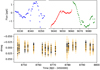 |
Fig. 1 Photometrie time series of GJ 832. Top panel: TESS (SAP) data from sectors 1 (blue), 27 (red), and 28 (green). The flux is given in parts per thousand (ppt). Bottom panel: ASH2 data using B (black) and V (orange) filters, which are given in differential magnitudes. |
3.1.2 UCLES
UCLES is mounted on the Anglo-Australian Telescope located at the Australian Astronomical Observatory. Its spectral resolution is 50 000 covering a wavelength range between 300 nm and 1100 nm. We added a total of 39 data points from UCLES obtained in a time span of 5465 days (from 1998 to 2013), and they are are publicly available (Wittenmyer et al. 2014) with a mean error of 2.59 m s−1.
3.1.3 PFS
We also included data from the PFS spectrograph installed in the 6.5 m Magellan Clay telescope located at Las Campanas Observatory in Chile. This echelle spectropgrah has a resolution of 80,000 over a wavelength range between 391 nm and 731 nm. A total of 16 PFS measurements are available (Wittenmyer et al. 2014) over 818 days (from 2011 to 2013), with an average RV uncertainty of 0.9 m s−1.
3.2 Photometric Data
We analysed photometric data from TESS (Ricker et al. 2016) and ASH2, which are displayed in Fig. 1.
3.2.1 ASH2
We include photometric CCD observations of GJ 832 collected with the robotic 40-cm telescope ASH2 located at the SPACEOBS observatory in San Pedro de Atacama, Chile. The 40 cm robotic telescope is operated by the Instituto de Astrofíŕìca de Andalucía (IAA, CSIC), which is equipped with a CCD camera STL 11000 2.7K × 4K, FOV 54 × 82 arcmin. A total of 633 measurements were collected, of which 316 were taken with the B filter and 317 with the V filter. The data were obtained over 17 nights spanning 52 days during the period from September to November 2019. The typical exposure times are 15 and 8 s for both filters. The typical photometric aperture radius used in the data reduction is 1.23″ pixel−1.
Only subframes with 40% of the total field of view (FOV) were used for an effective FOV of 21.6 × 32.8 arcmin. All CCD measurements were obtained by the method of synthetic aperture photometry without pixel binning. Each CCD frame was corrected in a standard way for dark and flat fielding. Different aperture sizes were also tested in order to choose the one that produces the light curve with the least dispersion. The nearby and relatively bright stars showing the lowest root mean square (RMS) flux scatter were selected as reference stars.
3.2.2 TESS
TESS observed GJ 382 in three Sectors, 1, 27, and 28, making a time span of 761 days. We made use of the light curves available on the Mikulski Archive for Space Telescopes (MAST1). GJ 832 does not have any transiting planets, but with this photometry data we can study the stellar variability. Since the pre-search data conditioning simple aperture photometry (PDCSAP) light curves are cleaned from long-term variabilities, we used simple aperture photometry (SAP) instead. To compensate for offsets between each SAP light curve, we used the light curves from each sector independently, making a total of three separate light curves.
To correct for systematics, we made use of the co-trending basis vectors (CBVs) that are generated in the PDC component of the TESS pipeline for each sector and CCD. These can be used to remove the most common systematic trends. The CBV correction is made in lightkurve (Lightkurve Collaboration 2018) using the CBVCorrector method in combination with the single-scale basis vector type which better preserves long-term signals.
4 Rotation Period
4.1 Spectroscopic Rotation Period
We calculated the following activity indicators from HARPS data: Hα, Hß, Hγ, Na I D, and S index. The latter is widely used to study activity (e.g. Duncan et al. 1991). Their generalised Lomb–Scargle (GLS) periodogram (Zechmeister & Kürster 2009) is displayed in Fig. 2. For the Hα, Hß, and Hγ indices, there are strong peaks at 45 days and around 200 days. As for the Na I D and S index, the largest peaks correspond to large periods between 1000 and 4000 days, and this may possibly be due to a long-term variation in the activity (stellar cycle type); the study of which is not within the scope of this article. There is also a significant peak at 37d in the sodium index, which is also present in the S index (2σ).
The stellar rotation period can be derived from S-index time series. As previous studies have shown (e.g. Haywood et al. 2014; Grunblatt et al. 2015; Rajpaul et al. 2015), the S index can be modelled using a Gaussian process (GP) regression.
In particular, the quasi-periodic kernel in a GP has a hyperparameter – the periodic component – attributable to the stellar rotation period. This kernel is described in Appendix A. We used the GP modelling capability of RadVel (Fulton et al. 2018) to perform this modelling. The priors on the hyperparameters correspond to the following uniform priors: in a range of 0 and 0.3 for the amplitude of correlations (η1); from 0 to 4000 days for the aperiodic timescale decay (η2); between 1 and 200 days for the periodic component (η3); and from 0 to 7 for the periodic timescale (η4). Readers can refer to Appendix B and Appendix D for more details on the priors and the Markov chain Monte Carlo (MCMC) results, respectively. Figure 3 shows the time series of the S index with the GP model. The periodic component of the quasi-periodic kernel has a value of  days (see Fig. B1), which is extremely close to the orbital period of putative planet c. Since stellar activity varies over time (and therefore also the activity indicators), we also modelled each HARPS campaign separately and retrieved a clear detection around 37 days for each dataset: 37.13 ± 2.03 days for HARPS and 35.99 ± 1.66 days for HARPS+, which is consistent with the periodicity obtained using the entire time span. From the S-index fit, the measurement of the stellar rotation period is improved by a factor of 6 with respect of the reported value by (Suárez Mascareño et al. 2015).
We also modelled the other activity tracers (Hα, Hß, Hγ, and Na D I) with a GP, using the same priors as in the S-index model. We found a clear rotation detection on the Na DI index, giving a result of 36.6 ± 1.2 days, which is in agreement with the S-index measurement. For the remaining activity indices, we could not retrieve a clear detection of the rotation period (see Fig. 2).
Since the time span is larger for the RV data than for the photometry and because the S index is widely used for modelling stellar activity, we used this measurement for the final value of the stellar rotation. It is confirmed with the photometry data, as is shown in the following sub-section.
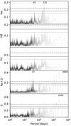 |
Fig. 2 GLS periodograms of the activity tracers. From top to bottom: Hα, Hß, Hγ, Na D I, and S index. The dashed, solid, and dotted horizontal lines represent the 0.3%, 4.6%, and 31.7% FAP levels, corresponding to a 3σ, 2σ, and 1σ detection threshold, respectively. |
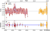 |
Fig. 3 S index time series modelled with a GP using a quasi-periodic kernel. Both HARPS (red squares) and HARPS+ (yellow circles) data are shown, a) Model showing the GP resulting from the median of the hyper-parameters’ posteriors (blue curve). The coloured zone depicts the model 1-σ confidence. Error bars account for the white noise included in the fit. b) Residual of the fit. |
4.2 Photometric Confirmation
We computed the GLS periodogram of the photometric data (TESS and ASH2), as shown in Fig. 4. There is a dominant peak around 35 days for every dataset, which could be the stellar rotation period as expected from the spectroscopic rotation period measurement.
To corroborate the rotation period, we also performed a GP regression on each photometric dataset. As with the activity analysis, we also made use of the quasi-periodic kernel. Further details as well as the posterior distribution of the parameters are given in Appendix A and Appendix B. Their resulting period distributions are shown in Fig. 5 along with the Na D I and S-index histograms. The periodic component of the ASH2 data is consistent with the stellar rotation period derived from the S index, whereas the TESS data show a wide distribution with a detection at  days, which is also in agreement with the rotation measurement. A single TESS sector is shorter than the rotation period, while the offset between sectors compromises the ability of the two consecutive sectors to discern the period (Fig. 1). Therefore, the photometric data confirm the result obtained from the S-index analysis.
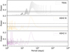 |
Fig. 4 GLS periodograms of GJ 832 from TESS (top) and ASH2 data using the B (center) and V (bottom) filters. The dashed, solid, and dotted horizontal lines are the same as in Fig. 2. |
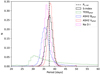 |
Fig. 5 Histogram of the periodic component of the quasi-periodic kernel η3, equivalent to the stellar rotation period. The vertical dashed line represents our measured value from the S index. We also depict distributions of the Na D I index and the photometric data from TESS and ASH2. |
5 RV Analysis
The RV dataset shows a clear and significant variation reaching 20 m s−1 with a mean error of 0.89 m s−1. We computed the GLS periodogram of the RVs, where we observe the most significant peak around 4000 days (planet b) far above the 3σ detection threshold (top panel of Fig. 6). We modelled the RVs using Pyaneti (Barragán et al. 2022).
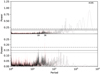 |
Fig. 6 GLS periodograms of GJ 832 from the RVs’ time series (top) and the RVs’ residual after removing the most significant signal (bottom). The old data are illustrated in red, whereas the new data (which includes 119 new measurements) are shown in black. The dashed, solid, and dotted horizontal lines are the same as in Fig. 2. |
5.1 1-Keplerian Model
For this model, we used uniform priors for the period around 3500 and 4200 days (see Table C.1 for more details about the priors). The largest peak in the residual periodogram corresponds to 18.7 days, which is equivalent to half of the stellar rotation found in Sect. 4.1, whereas the 35 days signal is not significant as it lies below 1σ (bottom panel of Fig. 6). We note that without our new HARPS data, the 35 days signal is significant.
We analysed the temporal stability of the signals present in RV residual after subtracting the model for planet b. We used the stacked Bayesian General Lomb–Scargle (sBGLS) periodogram formulated by (Mortier & Collier Cameron 2017). This enables us to discriminate stellar activity signals from planetary signals as active zones may not be stable over time in amplitude and phase because they appear or disappear at different regions of the stellar surface, while planetary signals are stable over time, thus being phase coherent. Hence, the power (or probability) with a planetary origin should always increase as more observations are added into the dataset.
The top panel of Fig. 7 shows the sBGLS periodogram of RV residual around 35 days. We note that as the number of observations grows, the probability around 35 days does not steadily increase; it starts to lose its significance when the last data points are added. The bottom panel shows the sBGLS periodogram around 18 days, the largest peak in the residual periodogram. Here we see the contrary: at the end of the dataset, this signal becomes more stable, which is in accordance with the GLS periodogram of the residual. The coherence of this latter signal favours a second planet at 18 days rather than at 35 days. A further analysis is performed in a 2-Keplerian model in the following section.
5.2 2-Keplerian Model
We also performed a 2-Keplerian model fit to check if the 35d and 18d signal could have a planetary origin. In this model, we considered the planet in the wide orbit (planet b) as one Keplerian, using the same priors as the 1-Keplerian model from Sect. 5.1, and then we added a second Keplerian using uniform priors on the period from 2 to 50 days. The rest of the priors are listed in Table C.2.
The best orbital solutions for this model gives an unclear detection (broad distribution and multiple peaks) for the second Keplerian, with a periodicity of  days. Therefore, a second Keplerian with a period of 18 or 15 days is not preferred for this model, suggesting that these signals do not correspond to planets. Motivated by this, simultaneous RV and activity indicator analyses are performed in the following section to determine whether these signals are related to stellar activity.
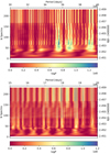 |
Fig. 7 sBGLS periodograms of the RVs’ residual (after subtracting the signal of planet b) centred around the 35d signal (top) and around 18 days (bottom), which corresponds to the largest peak on the residual periodogram. The number of observations is plotted against the period, whereas the colour bar indicates the logarithm of the probability. |
6 RV and Activity Indicators
We analysed the RVs alongside the activity indices Hα, Na D I, and the S index; each were analysed independently. Since we only have the activity indices from HARPS, we only used the RV measurements from this instrument to perform a simultaneous modelling with the same time series. The number of data points and the high precision of these measurements make this approach informative. We used 344 HARPS data points (172 RV measurements and the corresponding 172 measurements of activity data).
We explored the full (hyper-)parameter space with the publicly available Monte Carlo (MC) nested sampler and Bayesian inference tool MultiNest v3.10 (e.g. Feroz et al. 2019), through the pyMultiNest wrapper (Buchner et al. 2014). We set up 1000 live points, a sampling efficiency of 0.3, and a tolerance on the Bayesian evidence of 0.5. To perform the GP regression, we used the package george (Ambikasaran et al. 2015), using the QP kernel. Model comparison was performed using the logarithm of the Bayesian evidence  provided by MultiNest. The model comparison was done between the models with the same dataset but with different numbers of Keplerians. In this sense, we fitted one Keplerian with activity indices and then performed another model adding a second Keplerian (using the same priors).
To reduce the computation time, we used two (out of four) hyper-parameters in common: the rotation period (unique value for the star) and the evolutionary time scale. The latter could be different for RVs and activity indices, but it does not impact the modelling of the planetary signal. The priors of these models are listed in Table E.1. Table 3 compares the results of this fitting. We see that for the models using the Na D I and Hα indices, there is strong evidence against the second Keplerian  . As for the model containing the S index, it still indicates that the 1-Keplerian model has to be strongly preferred
  .
.
Moreover, for all the models, the stellar rotation period is detected around 36 days, as seen in Table 3. Additionally, in the case of two Keplerians, the models do not succeed at adjusting data where one of the planets has an orbital period periodicity around 35 days. Instead, a broad distribution (with many peaks) around 29 days is detected (P2 in Table 3), which is in agreement with our finding in Sect. 5.2 when we modelled two Keplerians (with no GP) for the entire dataset. In all the model cases, the fit of planet b stays unaffected, indicating this is a robust detection.
7 Best Model
Since the model comparison prefers only one Keplerian, we can update the orbital parameters of planet b. We did this by modelling one Keplerian with a GP with Pyaneti (Barragán et al. 2022), as we know from the previous section that the GP fits the stellar activity. We used the entire datasets (not only HARPS) since the UCLES and PFS data increase the time span and therefore the parameters for the wide-orbit planet are better determined. The model is displayed in Fig. 8 and the orbital values are shown in Table 4. The priors are listed in Table F.1 and the posterior distributions are shown in Fig. F1.
8 Discussion
Our results differ from previous studies of this system as we added 119 new HARPS spectra, making a total of 172 RV measurements. We also incorporated photometric observations. (Wittenmyer et al. 2014) performed their analysis with a total of 109 RV spectra when reporting on planet c. When analysing this set of data, after performing a 1-Keplerian fit to the planet in the outer orbit, we also found a significant (3σ) signal around 35 days in the residual. However, as we added the new HARPS data, this signal has lost its significance and does not even reach the detection threshold (bottom panel of Fig. 6) and it is only with the new HARPS RV data that we are able to determine the true origin of the 35 days signal. This is particularly noticeable for the addition of the RedDots data (56 RV measurements) which were taken with approximately nightly cadence to minimise sources of correlated noise and to be able to quantify the evolution of stellar activity features (for more details, see Jeffers et al. 2020).
Before we come to a final conclusion, we discuss the possibility that we have a planet with an orbital period close to the stellar rotation period. For example, K2-18 b (Sarkis et al. 2018) is an 8.5 M⊕ planet in a 32 days orbit around an M dwarf with a rotational period of 39 days. With RV measurements alone, the planetary signal is difficult to disentangle from the rotational modulation. Without the transit detection, this planet would have been undetected. A commensurability between planetary orbit and stellar rotation seems to be possible. Similarly, the K2-3 d planet was discovered by transits (Crossfield et al. 2015) with an orbital period around 44.5 days, whereas the stellar rotation period is around 40 days (Damasso et al. 2018). This planet is also not detectable using RV data (e.g. Almenara et al. 2015; Damasso et al. 2018), being challenging to disentangle between the signals from stellar activity and the planet, which is a different scenario than GJ 832 c.
Another case corresponds to HD 192263 b (Santos et al. 2000), a giant planet discovered by RV with an orbital period around 24days. This planet was discarded due to the proximity of the planetary orbital period and the stellar rotation (Henry et al. 2002), but it was re-analysed with photometry and bisector measurements (Santos et al. 2003), corroborating the presence of the planet. The RV variation showed stability (which is not the case for GJ 832 c) and the photometry showed variability. The planetary orbital period and stellar variability was disentangled (Dragomir et al. 2012), attributing a photometric variability of 23 days to the stellar rotation.
A recent example is AUMic b with a 7:4 commensurability (Szabó et al. 2021). (Walkowicz & Basri 2013) also found an over density of 1:1 and 2:1 ratios between rotational and orbital periods in the Kepler sample, but only for planets with a radius above about 6 R⊕. The radius of the planet candidate GJ 832c is probably below that threshold, which makes it unlikely that we have a situation comparable to this case.
Furthermore, both (Vanderburg et al. 2016) and (Newton et al. 2016) show that the RV jitter from stellar rotation coincides with the periodrange of Keplerian orbits in the HZ around M dwarfs. This is indeed the case for the putative planet GJ 832 c.
Model comparison table from the simultaneous RV and activity index fits.
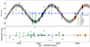 |
Fig. 8 1-Keplerian with GP orbital model for GJ 832 using HARPS (blue), HARPS+ (orange), UCLES (green), and PFS (red) datasets. Top panel: best fit for the planetary signal and GP (black solid line). The dark grey shaded regions correspond to the 1-and 2-σ credible intervals, respectively. Bottom panel: residual of the model. |
Updated orbital solutions of GJ 832 b.
9 Summary and Conclusions
We have collected a significantly expanded dataset for GJ 832, comprised of new RV, activity, and photometric data. We have thus used several statistical tools to study the exoplanetary system, its rotation, and stellar activity. We summarise our results below.
We measured the stellar rotation period from the spectroscopic activity indices, with a resulting value of
 days. This overlaps within uncertainties with the 35 days signal reported to be a planet. This result agrees with the photometric data.
The GLS periodogram from the RV residual detects a significant signal at 18.7 days, which corresponds to half of the rotation period.
The residual stacked Bayesian GLS periodogram shows the 35d signal is incoherent and does not persist, contrary to the expected behaviour of a signal induced by a planetary companion.
The 2-Keplerian models do not find a planet with a periodicity around 35 days.
The RV and activity index models (using HARPS data) prefers a 1-Keplerian model under a Bayesian framework.
These results provide a new characterisation and interpretation of stellar activity features for GJ 832. They allow us to conclude with confidence that the previously reported planet corresponding to the 35days signal is an artefact of stellar activity.
Acknowledgments
Acknowledgements. We thank the referee for the constructive comments that improved the quality of the manuscript. P.G. acknowledges research funding from CONICYT project 22181925. N.A.-D. acknowledges the support of FONDECYT project 3180063. SVJ acknowledges the support of the DFG priority programme SPP 1992 “Exploring the Diversity of Extrasolar Planets (JE 701/5-1). F.D.S. acknowledges support from a Marie Curie Action of the European Union (grant agreement 101030103). R.E.M. gratefully acknowledges support by the ANID BASAL projects ACE210002 and FB210003 and FONDECYT 1190621. Y.T. acknowledges the support of DFG priority program SPP 1992 ‘Exploring the Diversity of Extrasolar Planets” (TS 356/3-1). J.R. Barnes and C.A. Haswell are funded by STFC under consolidated grant ST/T000295/1. We acknowledge financial support from the Spanish Agencia Estatal de Investigación of the Ministerio de Ciencia, Innovación y Universidades through projects PID2019-109522GB-C52, PID2019-107061GB-C64, PID2019-110689RB-100 and the Centre of Excellence ‘Severo Ochoa’ Instituto de Astrofísica de Andalucía (SEV-2017-0709). We acknowledge the support by FCT – Fundação para a Ciência e a Tecnologia through national funds and by FEDER through COM-PETE2020 – Programa Operacional Competitividade e Internacionalização by these grants: UID/FIS/04434/2019; UIDB/04434/2020; UIDP/04434/2020; PTDC/FIS-AST/32113/2017 & POCI-01-0145-FEDER-032113; PTDC/FISAST/28953/2017 & POCI-01-0145-FEDER-028953. This work made use of RadVel (Fulton et al. 2018), Pyaneti (Barragán et al. 2022), MultiNest v3.10 (e.g. Feroz et al. 2019)), pyMultiNest wrapper (Buchner et al. 2014), george (Ambikasaran et al. 2015), and lightkurve (Lightkurve Collaboration 2018). This research includes publicly available data from the Mikulski Archive for Space Telescopes (MAST) from the TESS mission, as well as data public data from HARPS, UCLES and PFS.
Appendix A GP model
GPs are used to model stochastic processes with some known properties but unknown functional forms. They allow us to model relationships that are not necessarily linear, and they are suitable to model physical processes since they can cover a wide range of functions that can fit the phenomenon. This is why GPs are appropriate to characterise signals of stellar activity: although there are many unknown parameters, we know that they are (quasi-) periodic as they are modulated by stellar rotation. A quasi-period kernel is used with a covariance matrix given by
![Mathematical equation: $\sum\limits_{ij} { = \eta _1^2\exp } \left[ { - {{{{\left| {{t_i} - {t_j}} \right|}^2}} \over {\eta _2^2}} - {{{{\sin }^2}\left( {{{\pi \left| {{t_i} - {t_j}} \right|} \over {\eta _3^2}}} \right)} \over {2\eta _4^2}}} \right]\,,$](/articles/aa/full_html/2022/08/aa43063-22/aa43063-22-eq26.png) (A.1)
(A.1)
where Σij represents the element of covariance matrix, that is to say the covariance between observations at ti and tj. The parameter η3 corresponds to the periodic component, which in this case is the stellar rotation. The other parameters are related to the correlation between the data points. The aperiodic timescale decay of the correlations is represented by η2, which parameterises the evolutionary timescale of the active regions responsible for the observed periodic modulation. The parameter η4 is the periodic scale and η1 is the amplitude of the correlations.
Appendix B Further Information on the Rotation Period Derivation
Appendix B.1 S index
Priors used in the S-index model with a GP.
Appendix B.2 Photometry
Priors used in the ASH2 GP model. The data were modelled separately (due to the different filters), but we used the same priors for both ASH2 models.
Priors used in the TESS GP model.
Priors of the 1-Keplerian model.
Appendix C Details on the Keplerian models
Priors of the 2-Keplerian model.
Appendix D Details on the MCMC analysis
For the S-index model using a GP, we used RADVEL, which runs an MCMC analysis. We used the default values (such as the number of MCMC walkers= 50, number of steps=10000, and number of ensembles=8). For more details, readers can refer to (Fulton et al. 2018). As stated in their paper, they used the Gelman-Rubin statistic for convergence by comparing the intra-and inter-chain variances, in which a value close to unity indicates the convergence of the chains, and checking them after every 50 steps.
For the Keplerian models (without activity indicators), we made use of PYANETI which also runs an MCMC analysis. We also used the default values (number of chains = 100, number of iterations =500, thin factor=10, and number of walkers=100) for these models. The convergence is reached when the Gelman criterion  is smaller than 1.02 for all the sampled parameters.
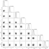 |
Fig. B1 Marginalised posterior distributions for the parameters of the GP. The physical parameter η3, indicates the stellar rotational period. |
Appendix E Details on the RV and activity index models
Summary of priors of the 1- and 2-Keplerian and activity index model (with GP).
Appendix F Details on the best model (1-Keplerian and GP)
Priors of the 1-Keplerian and GP model.
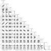 |
Fig. F1 Corner plot from the 1-Keplerian and GP model. |
References
- Almenara, J. M.,Astudillo-Defru, N.,Bonfils, X., et al. 2015, A&A, 581,A7 [Google Scholar]
- Ambikasaran, S.,Foreman-Mackey, D.,Greengard, L.,Hogg, D. W.,&O’Neil, M. 2015, IEEE Trans. Pattern Anal. Mach. Intell., 38,252 [Google Scholar]
- Anglada-Escudé, G.,&Butler, R. P. 2012, ApJS, 200,15 [CrossRef] [Google Scholar]
- Astudillo-Defru, N.,Delfosse, X.,Bonfils, X., et al. 2017a, A&A, 600,A13 [NASA ADS] [CrossRef] [EDP Sciences] [Google Scholar]
- Astudillo-Defru, N.,Forveille, T.,Bonfils, X., et al. 2017b, A&A, 602,A88 [NASA ADS] [CrossRef] [EDP Sciences] [Google Scholar]
- Bailey, J.,Butler, R. P.,Tinney, C. G., et al. 2009, ApJ, 690,743 [NASA ADS] [CrossRef] [Google Scholar]
- Barnes, J. R.,Jeffers, S. V.,&Jones, H. R. A. 2011, MNRAS, 412,1599 [NASA ADS] [CrossRef] [Google Scholar]
- Barragán, O.,Aigrain, S.,Rajpaul, V. M.,&Zicher, N. 2022, MNRAS, 509,866 [Google Scholar]
- Boisse, I.,Bouchy, F.,Hébrard, G., et al. 2011, A&A, 528,A4 [NASA ADS] [CrossRef] [EDP Sciences] [Google Scholar]
- Bonfils, X.,Mayor, M.,Delfosse, X., et al. 2007, A&A, 474,293 [NASA ADS] [CrossRef] [EDP Sciences] [Google Scholar]
- Bouchy, F.,Pepe, F.,&Queloz, D. 2001, A&A, 374,733 [NASA ADS] [CrossRef] [EDP Sciences] [Google Scholar]
- Buchner, J.,Georgakakis, A.,Nandra, K., et al. 2014, A&A, 564,A125 [NASA ADS] [CrossRef] [EDP Sciences] [Google Scholar]
- Crane, J. D.,Shectman, S. A.,&Butler, R. P. 2006, Society of Photo-Optical Instrumentation Engineers (SPIE) Conference Series, 6269, The Carnegie Planet Finder Spectrograph,626931 [Google Scholar]
- Crossfield, I. J. M.,Petigura, E.,Schlieder, J. E., et al. 2015, ApJ, 804,10 [NASA ADS] [CrossRef] [Google Scholar]
- Damasso, M.,Bonomo, A. S.,Astudillo-Defru, N., et al. 2018, A&A, 615,A69 [NASA ADS] [CrossRef] [EDP Sciences] [Google Scholar]
- Desidera, S.,Gratton, R. G.,Endl, M., et al. 2004, A&A, 420,L27 [NASA ADS] [CrossRef] [EDP Sciences] [Google Scholar]
- Diego, F.,Charalambous, A.,Fish, A. C.,&Walker, D. D. 1990, Society of Photo-Optical Instrumentation Engineers (SPIE) Conference Series, 1235, Final tests and commissioning of the UCL echelle spectrograph, ed.D. L. Crawford,562 [Google Scholar]
- Dragomir, D.,Kane, S. R.,Henry, G. W., et al. 2012, ApJ, 754,37 [NASA ADS] [CrossRef] [Google Scholar]
- Duncan, D. K.,Vaughan, A. H.,Wilson, O. C., et al. 1991, ApJS, 76,383 [NASA ADS] [CrossRef] [Google Scholar]
- Duvvuri, G. M.,Sebastian Pineda, J.,Berta-Thompson, Z. K., et al. 2021, ApJ, 913,40 [NASA ADS] [CrossRef] [Google Scholar]
- Feroz, F.,Hobson, M. P.,Cameron, E.,&Pettitt, A. N. 2019, Open J. Astrophys., 2,10 [NASA ADS] [CrossRef] [Google Scholar]
- Fontenla, J. M.,Linsky, J. L.,Witbrod, J., et al. 2016, ApJ, 830,154 [NASA ADS] [CrossRef] [Google Scholar]
- Fulton, B. J.,Petigura, E. A.,Blunt, S.,&Sinukoff, E. 2018, PASP, 130,044504 [NASA ADS] [CrossRef] [Google Scholar]
- Gaia Collaboration 2018, VizieR Online Data Catalog: I/345 [Google Scholar]
- Gomes da Silva, J.,Santos, N. C.,Bonfils, X., et al. 2011, A&A, 534,A30 [NASA ADS] [CrossRef] [EDP Sciences] [Google Scholar]
- Grunblatt, S. K.,Howard, A. W.,&Haywood, R. D. 2015, ApJ, 808,127 [NASA ADS] [CrossRef] [Google Scholar]
- Guinan, E. F.,Engle, S. G.,&Durbin, A. 2016, ApJ, 821,81 [NASA ADS] [CrossRef] [Google Scholar]
- Haywood, R. D.,Collier Cameron, A.,Queloz, D., et al. 2014, MNRAS, 443,2517 [NASA ADS] [CrossRef] [Google Scholar]
- Henry, G. W.,Donahue, R. A.,&Baliunas, S. L. 2002, ApJ, 577,L111 [NASA ADS] [CrossRef] [Google Scholar]
- Houdebine, E. R. 2010, MNRAS, 407,1657 [NASA ADS] [CrossRef] [Google Scholar]
- Huélamo, N.,Figueira, P.,Bonfils, X., et al. 2008, A&A, 489,L9 [NASA ADS] [CrossRef] [EDP Sciences] [Google Scholar]
- Jeffers, S. V.,Schöfer, P.,Lamert, A., et al. 2018, A&A, 614,A76 [NASA ADS] [CrossRef] [EDP Sciences] [Google Scholar]
- Jeffers, S. V.,Dreizler, S.,Barnes, J. R., et al. 2020, Science, 368,1477 [NASA ADS] [CrossRef] [Google Scholar]
- Kasting, J. F.,Whitmire, D. P.,&Reynolds, R. T. 1993, Icarus, 101,108 [NASA ADS] [CrossRef] [Google Scholar]
- Koen, C.,Kilkenny, D.,van Wyk, F.,&Marang, F. 2010, MNRAS, 403,1949 [NASA ADS] [CrossRef] [Google Scholar]
- Kruczek, N.,France, K.,Evonosky, W., et al. 2017, ApJ, 845,3 [NASA ADS] [CrossRef] [Google Scholar]
- Lightkurve Collaboration (Cardoso, J. V. D. M., et al.) 2018, Lightkurve: Kepler and TESS time series analysis in Python, Astrophysics Source Code Library [record ascl:1812.013] [Google Scholar]
- Lo Curto, G.,Pepe, F.,Avila, G., et al. 2015, The Messenger, 162,9 [NASA ADS] [Google Scholar]
- Maldonado, J.,Affer, L.,Micela, G., et al. 2015, A&A, 577,A132 [NASA ADS] [CrossRef] [EDP Sciences] [Google Scholar]
- Mayor, M.,Pepe, F.,Queloz, D., et al. 2003, The Messenger, 114,20 [NASA ADS] [Google Scholar]
- Mortier, A.,&Collier Cameron, A. 2017, A&A, 601,A110 [NASA ADS] [CrossRef] [EDP Sciences] [Google Scholar]
- Newton, E. R.,Irwin, J.,Charbonneau, D.,Berta-Thompson, Z. K.,&Dittmann, J. A. 2016, ApJ, 821,L19 [NASA ADS] [CrossRef] [Google Scholar]
- Peacock, S.,Barman, T.,Shkolnik, E. L., et al. 2019, ApJ, 886,77 [NASA ADS] [CrossRef] [Google Scholar]
- Queloz, D.,Henry, G. W.,Sivan, J. P., et al. 2001, A&A, 379,279 [NASA ADS] [CrossRef] [EDP Sciences] [Google Scholar]
- Rajpaul, V.,Aigrain, S.,Osborne, M. A.,Reece, S.,&Roberts, S. 2015, MNRAS, 452,2269 [NASA ADS] [CrossRef] [Google Scholar]
- Reiners, A.,Joshi, N.,&Goldman, B. 2012, AJ, 143,93 [NASA ADS] [CrossRef] [Google Scholar]
- Ricker, G. R.,Vanderspek, R.,Winn, J., et al. 2016, in Society of Photo-Optical Instrumentation Engineers (SPIE) Conference Series, 9904, Space Telescopes and Instrumentation 2016: Optical, Infrared, and Millimeter Wave, eds.H. A. MacEwen,G. G. Fazio,M. Lystrup,N. Batalha,N. Siegler,&E. C. Tong,99042B [Google Scholar]
- Robertson, P.,&Mahadevan, S. 2014, ApJ, 793,L24 [NASA ADS] [CrossRef] [Google Scholar]
- Robertson, P.,Roy, A.,&Mahadevan, S. 2015, ApJ, 805,L22 [NASA ADS] [CrossRef] [Google Scholar]
- Santos, N. C.,Mayor, M.,Naef, D., et al. 2000, A&A, 356,599 [NASA ADS] [Google Scholar]
- Santos, N. C.,Udry, S.,Mayor, M., et al. 2003, A&A, 406,373 [NASA ADS] [CrossRef] [EDP Sciences] [Google Scholar]
- Santos, N. C.,Mortier, A.,Faria, J. P., et al. 2014, A&A, 566,A35 [NASA ADS] [CrossRef] [EDP Sciences] [Google Scholar]
- Sarkis, P.,Henning, T.,Kürster, M., et al. 2018, AJ, 155,257 [NASA ADS] [CrossRef] [Google Scholar]
- Sebastian, D.,Gillon, M.,Ducrot, E., et al. 2021, A&A, 645,A100 [NASA ADS] [CrossRef] [EDP Sciences] [Google Scholar]
- Suárez Mascareño, A.,Rebolo, R.,González Hernández, J. I.,&Esposito, M. 2015, MNRAS, 452,2745 [CrossRef] [Google Scholar]
- Szabó, G. M.,Gandolfi, D.,Brandeker, A., et al. 2021, A&A, 654,A159 [NASA ADS] [CrossRef] [EDP Sciences] [Google Scholar]
- Vanderburg, A.,Plavchan, P.,Johnson, J. A., et al. 2016, MNRAS, 459,3565 [NASA ADS] [CrossRef] [Google Scholar]
- Vaughan, A. H.,Preston, G. W.,&Wilson, O. C. 1978, PASP, 90,267 [NASA ADS] [CrossRef] [Google Scholar]
- Walkowicz, L. M.,&Basri, G. S. 2013, MNRAS, 436,1883 [NASA ADS] [CrossRef] [Google Scholar]
- Wittenmyer, R. A.,Tuomi, M.,Butler, R. P., et al. 2014, ApJ, 791,114 [NASA ADS] [CrossRef] [Google Scholar]
- Zechmeister, M.,&Kürster, M. 2009, A&A, 496,577 [CrossRef] [EDP Sciences] [Google Scholar]
- Zechmeister, M.,Reiners, A.,Amado, P. J., et al. 2018, A&A, 609,A12 [NASA ADS] [CrossRef] [EDP Sciences] [Google Scholar]
All Tables
Priors used in the ASH2 GP model. The data were modelled separately (due to the different filters), but we used the same priors for both ASH2 models.
Summary of priors of the 1- and 2-Keplerian and activity index model (with GP).
All Figures
|
Fig. 1 Photometrie time series of GJ 832. Top panel: TESS (SAP) data from sectors 1 (blue), 27 (red), and 28 (green). The flux is given in parts per thousand (ppt). Bottom panel: ASH2 data using B (black) and V (orange) filters, which are given in differential magnitudes. |
| In the text | |
|
Fig. 2 GLS periodograms of the activity tracers. From top to bottom: Hα, Hß, Hγ, Na D I, and S index. The dashed, solid, and dotted horizontal lines represent the 0.3%, 4.6%, and 31.7% FAP levels, corresponding to a 3σ, 2σ, and 1σ detection threshold, respectively. |
| In the text | |
|
Fig. 3 S index time series modelled with a GP using a quasi-periodic kernel. Both HARPS (red squares) and HARPS+ (yellow circles) data are shown, a) Model showing the GP resulting from the median of the hyper-parameters’ posteriors (blue curve). The coloured zone depicts the model 1-σ confidence. Error bars account for the white noise included in the fit. b) Residual of the fit. |
| In the text | |
|
Fig. 4 GLS periodograms of GJ 832 from TESS (top) and ASH2 data using the B (center) and V (bottom) filters. The dashed, solid, and dotted horizontal lines are the same as in Fig. 2. |
| In the text | |
|
Fig. 5 Histogram of the periodic component of the quasi-periodic kernel η3, equivalent to the stellar rotation period. The vertical dashed line represents our measured value from the S index. We also depict distributions of the Na D I index and the photometric data from TESS and ASH2. |
| In the text | |
|
Fig. 6 GLS periodograms of GJ 832 from the RVs’ time series (top) and the RVs’ residual after removing the most significant signal (bottom). The old data are illustrated in red, whereas the new data (which includes 119 new measurements) are shown in black. The dashed, solid, and dotted horizontal lines are the same as in Fig. 2. |
| In the text | |
|
Fig. 7 sBGLS periodograms of the RVs’ residual (after subtracting the signal of planet b) centred around the 35d signal (top) and around 18 days (bottom), which corresponds to the largest peak on the residual periodogram. The number of observations is plotted against the period, whereas the colour bar indicates the logarithm of the probability. |
| In the text | |
|
Fig. 8 1-Keplerian with GP orbital model for GJ 832 using HARPS (blue), HARPS+ (orange), UCLES (green), and PFS (red) datasets. Top panel: best fit for the planetary signal and GP (black solid line). The dark grey shaded regions correspond to the 1-and 2-σ credible intervals, respectively. Bottom panel: residual of the model. |
| In the text | |
|
Fig. B1 Marginalised posterior distributions for the parameters of the GP. The physical parameter η3, indicates the stellar rotational period. |
| In the text | |
|
Fig. F1 Corner plot from the 1-Keplerian and GP model. |
| In the text | |
Current usage metrics show cumulative count of Article Views (full-text article views including HTML views, PDF and ePub downloads, according to the available data) and Abstracts Views on Vision4Press platform.
Data correspond to usage on the plateform after 2015. The current usage metrics is available 48-96 hours after online publication and is updated daily on week days.
Initial download of the metrics may take a while.