| Issue |
A&A
Volume 618, October 2018
|
|
|---|---|---|
| Article Number | A20 | |
| Number of page(s) | 4 | |
| Section | Stellar atmospheres | |
| DOI | https://doi.org/10.1051/0004-6361/201833060 | |
| Published online | 08 October 2018 | |
A new method to compute limb-darkening coefficients for stellar atmosphere models with spherical symmetry: the space missions TESS, Kepler, CoRoT, and MOST⋆,⋆⋆
1
Instituto de Astrofísica de Andalucía CSIC, Apartado 3004, 18080 Granada, Spain
e-mail: claret@iaa.es
2
Dept. Física Teórica y del Cosmos, Universidad de Granada, Campus de Fuentenueva s/n, 10871 Granada, Spain
Received:
20
March
2018
Accepted:
15
April
2018
Aims. One of the biggest problems we can encounter while dealing with the limb-darkening coefficients for stellar atmospheric models with spherical symmetry is the difficulty of adjusting both the limb and the central parts simultaneously. In particular, the regions near the drop-offs are not well reproduced for most models, depending on Teff, log g, or wavelength. Even if the law with four terms is used, these disagreements still persist. Here we introduce a new method that considerably improves the description of both the limb and the central parts and that will allow users to test models of stellar atmospheres with spherical symmetry more accurately in environments such as exoplanetary transits, eclipsing binaries, etc.
Methods. The method introduced here is simple. Instead of considering all the μ points in the adjustment, as is traditional, we consider only the points until the drop-off (μcri) of each model. From this point, we impose a condition I(μ)/I(1) = 0. All calculations were performed by adopting the least-squares method.
Results. The resulting coefficients using this new method reproduce the intensity distribution of the PHOENIX spherical models (COND and DRIFT) quite well for the photometric systems of the space missions TESS, Kepler, CoRoT, and MOST. The calculations cover the following ranges of local gravity and effective temperatures: 2.5 ≤ log g ≤ 6.0 and 1500 K ≤ Teff ≤ 12 000 K. The new spherical coefficients can easily be adapted to the most commonly used light curve synthesis codes.
Key words: binaries: eclipsing / stars: atmospheres / planetary systems
Additional calculations for other photometric systems and/or other bi-parametric laws can be performed on request.
Tables 2–17 are only available in electronic form at the CDS via anonymous ftp to cdsarc.u-strasbg.fr (130.79.128.5) or via http://cdsarc.u-strasbg.fr/viz-bin/qcat?J/A+A/618/A20
© ESO 2018
1. Introduction
The difficulty of finding good numerical adjustments simultaneously for the angular distribution of specific intensities of spherical stellar atmospheres models to derive limb-darkening coefficients (LDC) is well known. To control this problem, some time ago some authors introduced the concept of quasi-spherical atmosphere. This concept allowed the use of spherical models, but without considering the regions near the limb (see e.g. Claret 2017). Another version of the quasi-spherical model was suggested by Wittkowskil et al. (2004): instead of truncating the models at a certain value of μ (often 0.10) the truncation was defined by searching for the maximum of the derivative of the specific intensity with respect to r and shifting the profile to this point, where  and μ is given by cos(γ), where γ is the angle between the line of sight and the outward surface normal. The resulting LDC reproduced the model intensities well, especially when a four-term law was adopted.
However, if we consider all values of μ, i.e. including the drop-off regions, not even the law with four terms was able to reproduce well the angular distribution of the specific intensities, except for a few values of Teff and log g. In this short paper, we introduce a new method that has proven able to reproduce well the angular distribution of the specific intensities of spherical models (including the region of the drop-offs) for the first time. The accuracy of the adjustments does not depend on the effective temperatures or log g. The paper is organized as follows. Section 2 introduces the new numerical method and the methodology. The results of the calculations are presented and discussed in Sect. 3.
2. Spherical symmetric LDC: a new numerical method
As commented in the Introduction, it has been difficult to reconcile good adjustments for the regions near the limb and for the central parts of spherical stellar atmosphere simultaneously. In this paper we introduce a simple but very effective method which is capable of describing with high precision the behaviour of specific intensity distribution of stellar model atmospheres with spherical symmetry (hereafter full spherical method, FSM). The resulting improvements are particularly important in the regions located near the limb. Often the traditional methods used to adjust spherical models considered all values of μ in the fitting process, except those adopting the quasi-spherical or r-method procedures, but by definition ignoring the regions near the limb (see Claret 2017 and references therein for a detailed discussion). Here, instead, we consider for the fitting process only the points until the drop-off (hereafter μcri) of each model. The value of μcri for each model was obtained by searching for the maximum of the derivative of the specific intensity with respect to r. From this point, we impose the condition I(μ)/I(1) ≡ 0.0. To guarantee a very precise fitting we describe the selected part of the disk the law introduced by Claret (2000) (1)
(1)
where I(1) is the specific intensity at the centre of the disk and ak are the corresponding LDC. We also carried out adjustments for the quadratic law, which is the most frequently used bi-parametric law (2)
(2)
where a and b are the corresponding quadratic LDC. The following models were used in this paper: PHOENIX-COND (Husser et al. 2013), and PHOENIX-DRIFT (Witte et al. 2009), both with spherical geometry (see Table 1). The PHOENIX-DRIFT models are suitable for very cold configurations, such as late-M, L, and T-type dwarfs since they were generated considering a detailed computation of high-temperature condensed clouds. These grids cover, together with solar abundances, the following ranges of local gravity and effective temperatures: 2.5 ≤ log g ≤ 6.0 and 1500 K ≤ Teff ≤ 12 000 K. The model atmosphere specifc intensities were convolved with the transmission curves of the four mentioned space missions, and all calculations were performed by adopting the least-squares method (LSM).
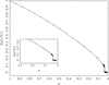 |
Fig. 1. Specific intensity distribution for a [Teff = 2600 K, log g = 5.0] PHOENIX-DRIFT spherical symmetric model. Asterisks represent the model intensities, while the dashed line denotes the traditional fitting with four terms and the continuous line the fitting using the FSM: Eq. (1); Log[A/H] = 0.0; Vξ = 2 km s−1; TESS photometric system; LSM calculations. |
3. Results and final remarks
In Fig. 1 we show the angular distribution of the specific intensity for a spherical model PHOENIX-DRIFT with Teff = 2600 K and log g = 5.0. We note that the traditional method gives a good adjustement but only up to μ ≈ 0.12, while the FSM provides a much better fitting for all values of μ, mainly near the limb. For a PHOENIX-COND [5600 K, 4.5] model the situation is similar to the previous model, except that the value of μ for which the traditional method gives a good fitting is changed to 0.2, instead of 0.12 (Fig. 2).
On the other hand, in Fig. 3 we can see the differences between models with the same log g and effective temperature [2800 K, 5.0] but computed with different input physics. For more details on the COND and DRIFT models, see Husser et al. (2013) and Witte et al. (2009), respectively. The respective μcri are similar, though the slope of the DRIFT model is larger.
The merit function is defined as (3)
(3)
where yi is the model intensity at point i, Yi the fitted function at the same point, N is the number of points, and M is the number of coefficients to be adjusted. This function is useful for evaluating the quality of the fittings. Figure 4 shows the superiority of the new FSM over the traditional one. In this figure the square root of the merit function for all PHOENIX-COND models is shown for the FSM (upper panel) and for the traditional method (lower panel). The panels are on the same scale to facilitate comparison. It is clear that the quality of the FSM fitting is much better than that obtained with the traditional method for any effective temperature or log g. On average, the merit function is approximately ten times smaller for the FSM. This scenario is similar for all photometric systems examined here and also for the monochromatic calculations.
The effects of the local gravity on the angular distribution of the specific intensities can be seen in Fig. 5 for the same input physics (PHOENIX-COND). As expected, the μcri for the giant star model is notoriously larger than for the main-sequence model at a fixed effective temperature. The effects of the effective temperature (for a fixed log g) on the intensity distribution are displayed in Fig. 6, the colder model showing more pronounced slope up to the μcri.
On the other hand, in Fig. 7 we can see the adjustment for the quadratic law (Eq. (2)), instead of Eq. (1) (see Fig. 1 for comparison). As expected, the goodness in this case it is a bit worse than that provided by Eq. (1), but it is still acceptable. Before adopting either Eqs. (1) or (2), the user should check the quality of the adjustment through the respective merit function.
In order to check the accuracy of the FSM, we also performed monochromatic calculations for several models scanning T eff and log g. We obtained the same results: the FSM is always superior to the traditional method and also describes the regions near the limb much more accurately. Among the advantages of the law (Eq. (1)) and the application of the FSM, we can list the following: (a) it uses a single law which is valid for the whole HR diagram; (b) it is capable of reproducing the specific intensity distribution very well, including the drop-offs; (c) the flux is conserved within a very small tolerance; (d) it is applicable to different photometric systems and to monochromatic values; and (e) it is applicable to different chemical compositions, effective temperatures, local gravities, and microturbulent velo-break cities.
The present spherical LDC can be used to study the effects of stellar atmosphere spherical models in the diverse environments where they are necessary, such as exoplanetary transits, eclipsing binaries, etc. The instruments installed on board the space missions, due to their high photometric accuracy, are especially suitable for trying to detect such effects. We performed calculations for four missions: TESS, Kepler, CoRoT, and MOST. Additional calculations for other photometric systems and/or other bi-parametric laws can be performed on request. The new coefficients and the condition I(μ)/I(1) ≡ 0.0 for μ < μcri can easily be adapted to the most commonly used light curve synthesis codes.
Finally, Table 1 summarizes the kind of data available at the CDS or directly from the author. Tables 2–5 contain the LDC for the TESS photometric system using the Eqs. (1) and (2) ([a1, a2, a3, a4], and [a, b]) as functions of the effective temperature and log g. The values of μcri are also given for each model in the tables as well as the merit function to guide the users when selecting the most suitable spherical LDC. Following the same pattern: Tables 6–9 for Kepler, Tables 10–13 for CoRoT, and Tables 14–17 for MOST. The even tables refer to the PHOENIX- DRIFT models while the odd ones refer to the PHOENIX- COND models. More details of the contents of Tables 2–17 can be found in the ReadMe file at CDS. Table A.1 shows an excerpt from Table 7 to help guide the reader.
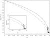 |
Fig. 3. Specific intensity distribution for spherical symmetric models. The continuous line represents the [Teff=2800 K, log g = 5.0] PHOENIX-COND model and the dashed line denotes the corresponding [Teff = 2800 K, log g = 5.0] PHOENIX-DRIFT. Asterisks represent the model intensities. Both fittings were performed with the FSM. Eq. (1); Log[A/H]= 0.0; Vξ = 2 km s−1; TESS photometric system; LSM calculations. |
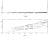 |
Fig. 4. Square root of the merit function adopting the FSM (first panel) and adopting the traditional method with four terms (second panel). Only the PHOENIX-COND models listed in Table 1 are displayed. To guarantee the homogeneity of the comparison the results of the DRIFT models, which were generated adopting a different input physics, are not displayed. Log[A/H] = 0.0; Vξ = 2 km s−1; TESS photometric system; LSM calculations. |
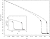 |
Fig. 5. Effects of the local gravity on the specific intensity distribution. The continuous line represents the [Teff = 5600 K, log g = 4.5] model and the dashed line [Teff = 5600 K, log g = 2.5]. Asterisks represent the model intensities. Both fittings were performed with the FSM. Eq. (1); PHOENIX-COND spherical symmetric models; Log[A/H] = 0.0; Vξ = 2 km s−1; Kepler photometric system; LSM calculations. |
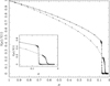 |
Fig. 6. Effects of the effective temperature on the specific intensity distribution. The continuous line represents the [Teff = 8000 K, log g = 4.5] model and the dashed line [Teff = 3000 K, log g = 4.5]. Asterisks represent the model intensities. Both fittings were performed with the FSM. PHOENIX-COND spherical symmetric models; Eq. (1); Log[A/H] = 0.0; Vξ = 2 km s−1; Kepler photometric system; LSM calculations. |
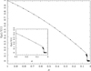 |
Fig. 7. Specific intensity distribution for a [Teff = 2600 K, log g = 5.0] PHOENIX-DRIFT spherical symmetric model. Asterisks represent the model intensities, while the continuous line represents the fitting using the FSM but adopting Eq. (2); Log[A/H] = 0.0; Vξ = 2 km s−1; TESS photometric system; LSM calculations. |
Limb-darkening coefficients for the space mission photometric system FSM.
Acknowledgments
I would like to thank G. Torres, J. Irwin, and B. Rufino for the helpful comments and T.-O. Husser and P. Hauschildt for providing the PHOENIX models. I also thank the anonymous referee who provided good suggestions for improving the manuscript. The Spanish MEC (AYA2015-71718-R and ESP2017-87676-C5-2-R) is gratefully acknowledged for its support during the development of this work. This research has made use of the SIMBAD database, operated at the CDS, Strasbourg, France, and of NASA’s Astrophysics Data System Abstract Service.
References
- Claret, A. 2000, A&A, 363, 1081 [NASA ADS] [Google Scholar]
- Claret, A. 2017, A&A, 600, A30 [NASA ADS] [CrossRef] [EDP Sciences] [Google Scholar]
- Husser, T.-O., Wende-von Berg, S., Dreizler, S., et al. 2013, A&A, 553, A6 [NASA ADS] [CrossRef] [EDP Sciences] [Google Scholar]
- Witte, S., Helling, Ch., & Hauschildt, P. H. 2009, A&A, 506, 1367 [NASA ADS] [CrossRef] [EDP Sciences] [Google Scholar]
- Wittkowskil, M., Aufdenberg, J. P., & Kervella, P. 2004, A&A, 413, 711 [NASA ADS] [CrossRef] [EDP Sciences] [Google Scholar]
Appendix A:
Supplementary table
Excerpt from Table 7.
All Tables
All Figures
|
Fig. 1. Specific intensity distribution for a [Teff = 2600 K, log g = 5.0] PHOENIX-DRIFT spherical symmetric model. Asterisks represent the model intensities, while the dashed line denotes the traditional fitting with four terms and the continuous line the fitting using the FSM: Eq. (1); Log[A/H] = 0.0; Vξ = 2 km s−1; TESS photometric system; LSM calculations. |
| In the text | |
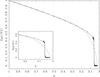 |
Fig. 2. As in Fig. 1, but for a [Teff = 5600 K, log g = 4.5] PHOENIX-COND spherical symmetric model. |
| In the text | |
|
Fig. 3. Specific intensity distribution for spherical symmetric models. The continuous line represents the [Teff=2800 K, log g = 5.0] PHOENIX-COND model and the dashed line denotes the corresponding [Teff = 2800 K, log g = 5.0] PHOENIX-DRIFT. Asterisks represent the model intensities. Both fittings were performed with the FSM. Eq. (1); Log[A/H]= 0.0; Vξ = 2 km s−1; TESS photometric system; LSM calculations. |
| In the text | |
|
Fig. 4. Square root of the merit function adopting the FSM (first panel) and adopting the traditional method with four terms (second panel). Only the PHOENIX-COND models listed in Table 1 are displayed. To guarantee the homogeneity of the comparison the results of the DRIFT models, which were generated adopting a different input physics, are not displayed. Log[A/H] = 0.0; Vξ = 2 km s−1; TESS photometric system; LSM calculations. |
| In the text | |
|
Fig. 5. Effects of the local gravity on the specific intensity distribution. The continuous line represents the [Teff = 5600 K, log g = 4.5] model and the dashed line [Teff = 5600 K, log g = 2.5]. Asterisks represent the model intensities. Both fittings were performed with the FSM. Eq. (1); PHOENIX-COND spherical symmetric models; Log[A/H] = 0.0; Vξ = 2 km s−1; Kepler photometric system; LSM calculations. |
| In the text | |
|
Fig. 6. Effects of the effective temperature on the specific intensity distribution. The continuous line represents the [Teff = 8000 K, log g = 4.5] model and the dashed line [Teff = 3000 K, log g = 4.5]. Asterisks represent the model intensities. Both fittings were performed with the FSM. PHOENIX-COND spherical symmetric models; Eq. (1); Log[A/H] = 0.0; Vξ = 2 km s−1; Kepler photometric system; LSM calculations. |
| In the text | |
|
Fig. 7. Specific intensity distribution for a [Teff = 2600 K, log g = 5.0] PHOENIX-DRIFT spherical symmetric model. Asterisks represent the model intensities, while the continuous line represents the fitting using the FSM but adopting Eq. (2); Log[A/H] = 0.0; Vξ = 2 km s−1; TESS photometric system; LSM calculations. |
| In the text | |
Current usage metrics show cumulative count of Article Views (full-text article views including HTML views, PDF and ePub downloads, according to the available data) and Abstracts Views on Vision4Press platform.
Data correspond to usage on the plateform after 2015. The current usage metrics is available 48-96 hours after online publication and is updated daily on week days.
Initial download of the metrics may take a while.