| Issue |
A&A
Volume 599, March 2017
|
|
|---|---|---|
| Article Number | A86 | |
| Number of page(s) | 11 | |
| Section | Astrophysical processes | |
| DOI | https://doi.org/10.1051/0004-6361/201629779 | |
| Published online | 03 March 2017 | |
Spiral-driven accretion in protoplanetary discs
III. Tridimensional simulations
1 Laboratoire AIM, Paris-Saclay, CEA/IRFU/SAp – CNRS – Université Paris Diderot, 91191 Gif-sur-Yvette Cedex, France
e-mail: This email address is being protected from spambots. You need JavaScript enabled to view it.
2 LERMA (UMR CNRS 8112), École Normale Supérieure, 75231 Paris Cedex, France
3 Univ. Grenoble Alpes, IPAG, 38000 Grenoble, France
4 CNRS, IPAG, 38000 Grenoble, France
Received: 23 September 2016
Accepted: 22 November 2016
Abstract
Context. Understanding how accretion proceeds in proto-planetary discs, and more generally, understanding their dynamics, is a crucial questions that needs to be answered to explain the conditions in which planets form.
Aims. The role that accretion of gas from the surrounding molecular cloud onto the disc may have on its structure needs to be quantified.
Methods. We performed tridimensional simulations using the Cartesian AMR code RAMSES of an accretion disc that is subject to infalling material.
Results. For the aspect ratio of H/R ≃ 0.15 and disc mass Md ≃ 10-2M⊙ used in our study, we find that for typical accretion rates of the order of a few 10-7M⊙ yr-1, values of the α parameter as high as a few 10-3 are inferred. The mass that is accreted in the inner part of the disc is typically at least 50% of the total mass that has been accreted onto the disc.
Conclusions. Our results suggest that external accretion of gas at moderate values onto circumstellar discs may trigger prominent spiral arms that are reminiscent of recent observations made with various instruments, and may lead to significant transport through the disc. If confirmed from observational studies, such accretion may therefore influence disc evolution.
Key words: instabilities / hydrodynamics / accretion, accretion disks
© ESO, 2017
1. Introduction
Accretion discs are ubiquitous in astrophysics because they are observed around stars and black holes, and as such, they have received considerable attention. In particular, it is widely admitted that local instabilities such as the magneto-rotational instability (MRI, e.g. Balbus 2003) or the gravitational instability (e.g. Lodato & Rice 2004) are responsible within different contexts for triggering the transport of angular momentum and mass. The conditions under which these mechanisms may work remain debated. It is unclear, for example, whether protostellar discs are sufficiently ionized for the MRI to operate efficiently (e.g. Lesur et al. 2014; Turner et al. 2014).
Mass-transferring binary systems are a well-studied type of disc, and it has early been recognized that the spiral shocks induced by the companion and the accretion is a source of external disturbances that can trigger significant accretion within the disc (Spruit 1987; Larson 1990; Vishniac & Diamond 1989). This has been confirmed by a series of numerical simulations (Sawada et al. 1987; Spruit et al. 1987; Rozyczka & Spruit 1993; Yukawa et al. 1997). In their recent study, Ju et al. (2016) considered the impact of spiral shocks in the presence of MRI turbulence and concluded that the former also play a significant role in this context.
In contrast, most studies have been studying proto-planetary discs in isolation because it is not yet clear whether these objects are still subject to infall from their surrounding parent molecular cloud. A notable exception are the studies that have addressed the question of discs that form out of their parent dense cores. The newly formed discs are usually massive, self-gravitating, and often strongly magnetized. It is generally accepted that angular momentum can be transported by the gravitational torque or by magnetic braking (e.g. Vorobyov & Basu 2008; Machida et al. 2010; Joos et al. 2012; Li et al. 2013; Vorobyov et al. 2015; Masson et al. 2016). For example, Vorobyov et al. (2015) performed a series of bidimensional studies of self-gravitating and viscous discs embedded in their parent cores, and showed that the infall of material has a drastic impact on their evolution. In particular, the angular momentum of the infalling material appears to be particularly important for the evolution.
To specifically investigate the role that infall may have on the disc, Lesur et al. (2015) performed bidimensional hydrodynamical simulations. The authors found that infall induces high values of α in the outer part of the disc and lower but non-negligeable values, on the order of a few 10-4 for an imposed accretion rate of about 10-7M⊙ yr-1, in the inner part of the disc where a plateau of constant α seems to be reached. It has also been shown that although slightly less efficient than non-axisymmetric inflows, axisymmetric flows quickly break up to form a spiral pattern and trigger non-stationary structures within the disc on even smaller scales.
It is now necessary to investigate this question in three dimensions, and for this purpose, we present here tridimensional numerical simulations of a disc that is subject to infall. Magnetic field and self-gravity are explicitly neglected at this stage. The second section of the paper describes the numerical setup, including initial and boundary conditions. It also presents a simulation of a non-accreting disc, which allows us to assess the initial conditions and the effect of numerical viscosity. In the third section, we present a simulation in detail and study the influence of numerical resolution. We provide some qualitative comparisons with previous analytical works. The influence of the strength of the accretion and quantitative comparison with bidimensional simulations is investigated in the fourth section. The influence of the geometry of the accretion flows and of the amount of angular momentum it carries is presented in the fifth section. Section 6 provides some discussions that link our results with recent observations of spiral patterns in transitional discs and their interpretation. The seventh section concludes the paper.
2. Tridimensional simulations: setup, resolution, and runs
We now describe the series of three-dimensional simulations we performed. In a companion paper (Lesur et al. 2015), we presented a series of two-dimensional runs.
2.1. General setup
2.1.1. Code
To perform our simulations, we employed the code RAMSES (Teyssier 2002), which is an adaptive mesh-refinement code working in Cartesian geometry and using finite-volume methods and Godunov solvers. Cylindrical or spherical geometries have traditionally been used in the context of disc studies because they ensure exact conservation of angular momentum. This is also the choice that has been made for the simulations presented in Lesur et al. (2015). However, these geometries also introduce singularities along the z-axis or at the origin, which requires specific treatments, while Cartesian codes do not present this difficulty.
2.1.2. Initial conditions
The initial state is an axisymmetric equilibrium between gravitational, centrifugal, and pressure forces. We adopted the locally isothermal approximation,  (1)where r is the cylindrical radius and Cs is the sound speed with
  . This approximation is supported by detailed models of the temperature structure of discs (D’Alessio et al. 1998; Armitage 2011), which specifically show that the dominant source of heating above 2 AU is the star irradiation. The mass of the central star is M∗ = 1, and the disc radius is equal to rd = 1/4 = Lb/ 8, where Lb = 2 is the size of the computational box. This choice ensures that the size of the disc is sufficiently small with respect to the computational box size, in such a way that it is not significantly influenced by boundary conditions. Below only the central part of the computational box is displayed. Therefore the disc initially occupies half of the image. In these units, the gravitational constant G is equal to 1. This ensures that the gravitational force is always 10 times larger than the pressure force in the radial direction. The disc aspect ratio is given by
  (2)where we used Ω ≃ r− 3/2 (since M∗ = 1 and G = 1). With this choice, the aspect ratio is therefore constant and equal to about 0.15.
Solving for the axial mechanical equilibrium, we obtain the density profile:  (3)where ρc is a free function of r that we have chosen to be equal to
  (4)The rotation curve is then obtained by requiring mechanical equilibrium in the radial direction,
  (5)The equilibrium solution is truncated at rd where the density is decreased to a value one hundred times lower. This causes the disc to expand initially. However, as shown below, the effect remains limited even in the absence of any external accretion.
The orbital time at the initial disc external radius, rd, is given by  (6)This constitutes the natural time units for the simulation results to which we refer here.
2.1.3. Inner boundary conditions
The central star is placed at the centre of the grid, and the corresponding gravitational force is directly added to the gas smoothing the r-2 dependence within a few computing cells. There is no sink of matter associated, and therefore the gas piles up in the vicinity of the star as the simulation evolves. Around the central star, mesh effects are very strong and the flow structure is much affected by the numerical resolution. As we quantitatively discuss below, the results can be considered as meaningful only at a certain distance from the central object.
The sound speed dependence, as stated by Eq. (1), leads to a singular behaviour near the z-axis. This creates spurious behaviours and leads to high velocities, which spoil the disc equilibrium. We therefore modified the sound speed at small radii, r. We essentially imposed that below a radius rd/ 10, the temperature is constant and equal to the value it has at this radius. Since, as described below, the numerical resolution drops at high altitude, we also slowly increased with height the radius inside which the temperature remains constant, which causes the isothermal surfaces to have a parabolic shape.
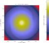 |
Fig. 1 Case of no accretion. Column density map. The disc has a radius of about r = 0.25. |
2.1.4. Outer boundary conditions
Since Cartesian coordinates are employed, the computational domain is a cubic box; this causes strong boundary effects. It would typically cause strong reflections and spurious m = 4 modes that affect the disc structure. To avoid these artefacts, the size of the disc was chosen to represent only 1/4 of the whole box size, as mentioned above, which is possible thanks to the AMR scheme of RAMSES. However, although it helps to reduce these effect, we find that they are still significant. Therefore we imposed a uniform density at every time step and a Keplerian velocity for every cell located at r> 0.9 (since the box size is Lb = 2, the boundary cells in the equatorial plan are located between r = 1 and  ) from the box centre. With this boundary condition, we found that in the absence of infall, the flow remains sufficiently symmetrical, as shown by Fig. 1.
2.1.5. Numerical resolution
To perform our calculations efficiently, we took advantage of the AMR scheme by using a coarse resolution outside the disc, that is to say, at radius r > rd = 1/4 and height larger than z > rd/ 2, while using a finer resolution inside the disc. For most of the runs, the resolution employed the AMR level, l = 10, inside the disc, which implies that the disc radius is described by 128 cells and the whole disc lies in a box of 256 × 256 × 128 cells. As discussed above, the aspect ratio of the disc is about 0.15. At the disc radius, the disc scale height is therefore described by about 40 cells. At a radius of r = rd/ 10, this number becomes equal to only 4 cells at a typical scale height. These simulations can therefore encompass a range of radius of the order of ≃5−10. We refer to this resolution as “standard” below.
To investigate the issue of numerical resolution, we also performed runs with a higher resolution in the inner part. The area located at r < 0.5 × rd is described using level l = 11, implying that at r = rd/ 10, the scale height is described by about 8 cells. We refer to this resolution as “high”. We note that at the same time, the radius at which the gas becomes isothermal was also reduced by a factor 2.
For all simulations, rd the resolution drops to level l = 8 above the disc radius. Then at radius r > 1.4rd = 0.35 it drops to level l = 7, and then at r > 2rd = 0.5, it reaches l = 6.
Typically, the simulations request about 10 000 (for the standard resolution) to about 100 000 cpu h (for the high resolution).
2.1.6. Accretion flow
To describe the external accretion, we imposed two types of inflow boundary conditions, one axisymmetric and one asymmetrical.
For the asymmetrical accretion scheme, the gas is injected from a circle of radius rd, contained in the (y,z) plane, and centred on x = −3.5rd,y = 0,and z = 0 at a radial velocity Uacc and with a density ρacc. The accreted gas possesses a specific angular momentum that is equal to either 0 or to  , that is to say, the angular momentum that corresponds to the Keplerian velocity at the disc radius, rd. The accretion velocity is expressed as a function of the sound speed at the boundary, which is equal to
  where Uacc = U0Cs/ 2. The accretion rate is thus given by
  (7)For the axisymmetrical accretion scheme, the gas is injected from a ring of radius 3.5rd and half-thickness rd. While the value of ρacc is unchanged, the values of Uacc are adjusted in such a way that the total accretion rate is identical to the asymmetrical case
  (8)Thus for given values of ρacc and U0, the value of Ṁ is identical for the two geometries.
Below we consider values of U0 = 0.5 and 2. To determine typical values of ρacc, we must refer to observational case. An efficient way to characterize external infall in accretion discs is given by the dimensionaless number, P, 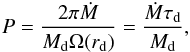 (9)that is to say, the ratio between the accreted mass (within the computing box) over one orbital period at r = rd and the disc mass. This parameter describes the speed at which mass is delivered into the disc per disc mass and typical disc timescale.
For a typical T Tauri star of 1 M⊙ and a radius rd = 100 AU, accretion rates onto the central star, Ṁacc, of the order of up to 10-7M⊙ yr-1 have been inferred (Muzerolle et al. 2005). If we assume that accretion onto the star is a consequence of external infall onto the disc, this suggests that the two accretion rates might be related and comparable. In the case of our simulations, with these numbers we have 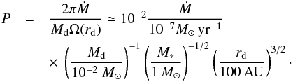 (10)With the density profile stated by Eq. (3) and
  , the mass of the disc initially is about 0.13. Since rd = 1/4, we find
 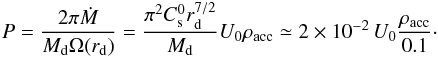 (11)In the following, we adopt ρacc = 0.1. We typically integrate during about 15 orbits at the outer radius. At rd/ 10, this roughly corresponds to about 500 orbits. During this amount of time and for the value U0 = 2, the total mass inside the computational box increases by about 30%. We stress, however, that the increase in disc mass, that is to say, inside the radius, rd, is 3−4 times lower than this value. This means that the effective mass flux that falls into the disc is 3−4 times lower than the analytical value stated by Eq. (7). This is because most of the mass added in the computational box piles up in the external medium where the density is initially low.
2.2. Runs performed
Summary of the different runs.
Table 1 summarizes the runs we performed and provides consistent labels. This set of simulations attempts to explore the influence of parameters for the accretion flow (velocity, density, symmetry, and angular momentum), and the numerical resolution.
The lowest value of P is 10-2, which for a 10-2M⊙ disc and a 1 M⊙ star corresponds to an accretion of about 10-7M⊙ s-1. This corresponds to a somewhat high accretion rate, but as explained below, the effective accretion rate onto the disc is typically 3−4 lower than this value. We note that reducing the accretion rate even more would be difficult because the numerical resolution (see Fig. 2) places constraints on the lowest flux that can be modelled.
2.3. Non-accreting case
As it is important to understand the limits of the numerical experiment we perform, we first carried out a run without accretion. Figure 1 shows a column density map at time 9.71 (we recall that the orbital time at the disc outer edge is about 0.75, which means that the disc has performed about 14 orbits). The disc remains smooth and symmetrical. There is a weak m = 2 pattern located near the disc radius r = 0.25. This is likely a consequence of the change in resolution there and the Cartesian mesh. The resulting column density, which is displayed in the top panel of Fig. 2 in four time steps, does not evolve very significantly. It slightly diminishes in the inner part below r< 0.03 because of the numerical resolution that becomes insufficient at small radii (see discussion in Sect. 2.1.5). It also increases in the outer part at radii larger than r> 0.3, that is to say, close to the disc radius. This is expected since the gas initially is out of equilibrium there. Overall, these effects remain fairly limited. We also computed the azimuthally averaged α parameter, which is defined as  (12)where δur and δuφ are the fluctuation of the radial and azimuthal velocities. α is displayed in the bottom panel of Fig. 2. After three to four orbits, it is below 10-3 for a radius of 0.03 <r< 0.3, that is to say, inside the disc, but sufficiently far from the centre. After eight to ten orbits, it has dropped even more and reaches values close to 10-4 almost everywhere in the disc. At small radii, r< 0.03, α increases to high values. This is clearly a consequence of the insufficient numerical resolution and is consistent with the column density variations.
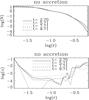 |
Fig. 2 Case of no accretion. Column density (top panel) and α value (bottom panel) as a function of the radius r. Typical variations remains limited, and the α values are below 10-3 and rapidly fall below 3 × 10⁻⁴. Note that at small radii (log (r) < −1.6), α increases to high values because of the low resolution. |
We conclude that the numerical setup we used permits us to investigate physical effects, which leads to transport characterized by α larger than about 10-4 in a region located between the disc radius, rd, and about rd/ 5. As reported below, this is indeed the case for the choice of parameters, namely the external accretion rate, that we consider.
3. Results for non-axisymmetric accretion of rotating gas
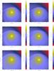 |
Fig. 3 Simulation ASR2 (asymmetrical accretion with U0 = 2 and standard resolution, left panels) and ASR2h (high resolution, right panels). Column density map at three different time steps. The disc initially has a radius of about r = 0.25. Note that the spiral pattern is remarkably stationary. |
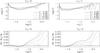 |
Fig. 4 Simulations ASR2 (left) and ASR2h (right). Top panels: α as a function of the radius r. Bottom panels: cumulated mass difference over total mass (see text). Solid lines at r = 0.25 represent the initial disc edge. |
3.1. Qualitative description
In this section, we present the simulation labelled as ASR2 in detail. It presents a non-asymmetric accretion flow that contains the same amount of angular momentum as the gas at the outer edge of the disc. It has an accretion parameter, P, that is about 4 × 10⁻². Figure 3 shows column density maps at three time steps (from about 4 to 15 orbits) and at two different resolutions (left panels: standard resolution, right panels: high resolution). The top panel shows various remarkable features. First of all, there is a prominent nearly stationary spiral arm that extends from x = −0.5, y = 0 to the disc. This is due to the incoming flow, which shocks the gas within the computational box (see further discussion in Sect. 6). This triggers the development of a prominent dense spiral arm within the disc, starting at about x = −0.2 and y = 0.15. Then, there is a second spiral arm that is slightly less prominent and more or less symmetrical to the first arm. Because the gas distribution around the disc is not symmetrical, the whole disc is clearly not symmetrical, indicating that m = 1 perturbations have been developing. This is at stark contrast with the non-accreting disc presented in Fig. 1.
The middle and bottom panels show later times. Clearly, the spiral patterns developed further and have propagated away, reaching a radius comparable to a few times the disc radius. This is reminiscent of the very prominent spiral pattern observed in numerical simulations of discs forming in class 0 protostars (e.g. Joos et al. 2012) and suggests that large-scale spiral patterns are a natural outcome of externally accreting discs.
3.2. Accreted mass and α parameter
To quantify the transport of mass that results from the large asymmetry induced by the incoming flow, we have computed the cumulated mass through the disc at various time steps as well as the mean α parameter.
The bottom panel of Fig. 4 shows the cumulated mass (that is to say, the mass contained within a cylinder of radius r) difference between a reference time (first time step quoted in the figure) and four later time steps, divided by the total mass within the box at the reference time (which is close to the mass within the disc). The four curves show similar features. First, the cumulated mass rapidly increases with radius in the region located outside the disc radius, r>rd. There is a clear break located approximately at the disc radius, rd ≃ 0.25, below which the cumulated mass varies less stiffly with radius. At log (r) ≃ −1.2, the cumulated mass remains constant with time, implying that no mass crosses this region. Below this radius, the cumulated mass difference slightly decreases with time, implying that the gas there is transported outwards (but not further than log (r) ≃ −1.2 where the difference in cumulated mass vanishes). This limit most likely represents the point above which the simulation results are dominated by grid effects, as anticipated in Sect. 2.1.5.
The α parameter is plotted in the top panel of Fig. 4. The general behaviour is similar to the no-accretion case (Fig. 2), α is large in the very inner part because of insufficient resolution, and in the disc outer part, where the external material is falling in. At intermediate radius, however, there is a plateau with values that increase with time to reach about 10-2. Since this value is about 30 times higher than the values obtained in the non-accretion case, this clearly shows that infall is responsible for the measured α.
3.3. Problem of numerical convergence
To verify the reliability of these simulations, we have performed higher resolution simulations. The right panels of Fig. 3 display the column density map at three time steps. A very similar pattern can be observed for the two resolutions, which apparently indicates that the simulations are not dominated by insufficient resolution effects inside the disc.
More quantitative comparisons are given in Fig. 4, where the right panels present the high -resolution run (ASR2h). The values of α are similar, although run ASR2 indicates slightly larger α at radius r< 0.1. The cumulated mass shown in the bottom panels of Fig. 4 is very similar in the outer part, that is, outside the disc (r> 0.25). The profiles are more different inside the disc, however. In particular, the cumulated mass vanishes at smaller radii for ASR2h than for ASR2. The profile of the former is also flatter than the profile of the latter. This is clearly an impact of the resolution, and it suggests that the limited resolution prevents accretion up to the centre.
Altogether, these results suggest that accretion triggered by the external flow is able to penetrate significantly inside the disc, probably at least down to a radius equal to ≃ rd/ 5. This number reflects the limit set by the highest resolution we could achieve, however. Typically, we find that with the present configuration, roughly 11% of the mass that has been injected in the box is accreted inside the disc at a radius below rd/ 2. At a radius below rd, this number can be larger than 20%, although defining the disc boundary is arbitrary because of the complexity of the flow in this region. This indicates that roughly 50% of the mass that is captured by the disc is able to penetrate at a radius smaller than rd/ 2.
3.4. Comparison between analytical and numerical solutions
 |
Fig. 5 Azimuthal profiles from simulation ASR2h at time t = 0.75 and at radius r = 0.08 (solid line), 0.14 (dotted), and 0.18 (dashed). Note that the density and the azimuthal velocity have been normalised such that their peak value is equal to 1. |
In an attempt to better understand the physical mechanism responsible for the transport of mass and angular momentum in the disc through the spiral-driven accretion, self-similar solutions in the r variables have been studied in Hennebelle et al. (2016) following the approach of Spruit (1987). These exact solutions of the inviscid fluid equations depend on the φ variable, the polar angle, and present two essential features. First of all, they undergo shocks, which play an essential role since this is where energy is dissipated, an essential feature for a system that transports angular momentum. Second, the radial velocity is changing sign with φ. This implies that there are both inward- and outward-bound mass fluxes. In particular, the latter is responsible for the outward-bound flux of angular momentum.
While self-similar solutions remain restricted by the heavy assumptions regarding their dependence, these two aspects constitute essential predictions that should be generic for any accretion disc driven by spiral waves, particularly in the absence of other forces such as self-gravity and magnetic field, which could exert a torque on the gas. To verify whether these features indeed play a role in the present simulations, Fig. 5 shows the azimuthal profiles of Ur, Uφ, and ρ at three different radii. The profiles clearly present some similarities with the self-similar solutions. In particular, the radial velocity, Ur, clearly changes sign. It remains negative in about one third of the angular distance and positive for the rest. Moreover, there are clear discontinuities, seen both in Ur and Uφ, that are similar to the shocks of the self-similar solutions (see Fig. 1 of Hennebelle et al. 2016). As expected, there are also significant differences. First, the dominant mode is m = 1, a clear consequence of the accretion pattern, which is also m = 1. No analytical solution was found for the case of m = 1. Second, there are multiple shock features instead of one. Finally, the density fields present more structure in the numerical simulations than in the analytical solutions. These differences are most likely consequences of the non-stationary nature of the numerical solutions.
4. Dependence on infall rate and comparison with bidimensional simulations
4.1. Dependence on infall rate
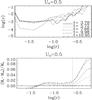 |
Fig. 6 Simulations ASR0.5h. α values and cumulated mass difference as a function of radius, r. |
To investigate the influence that infall has on the disc dynamics, we show a lower accretion rate that is characterized by an infall velocity equal to U0 = 0.5. As shown by Eqs. (10), (11), this corresponds to an accretion rate inside the computation box of about 10-7M⊙ yr-1. The effective accretion rate for the disc is ≃5 times smaller since, as we explained, most of the mass does not fall into the disc and remains in the surrounding region. The corresponding α profile and cumulative mass distribution are shown in Fig. 6. The values of α vary from a few 10-3 at log r = −0.9 to about 10-3 at log r = −1.3 at time 10.95. We note that these values fluctuate in particular at time 9.98, where they are typically twice lower (for log r > −1.3). For comparison, the α values for U0 = 2 are about four times higher with values of the order of 5 × 10⁻³ at log r = −1.3 and almost 10-2 at log r = −0.9.
As expected, the cumulated mass is also lower with U0 = 0.5. Its value at time 10.95 and at radii log r = −0.9 is about 1.5 × 10⁻³, while at similar time and radius it is about 5.5 × 10⁻³ for U0 = 4, that is to say, roughly four times higher. The mass accreted inside the disc (at log r < −1) is about 20% of the total mass injected in the computational box. Interestingly, the profile of the cumulated mass is fairly flat, which indicates that most of the mass accreted within the disc is transferred inwards.
4.2. Comparison with the 2D simulations
In their 2D simulations, Lesur et al. (2015) estimated that for an accretion rate of 10-7M⊙ yr-1, the asymmetrical case with rotation leads to values of α of about 4 × 10⁻⁴, which is therefore two to three times lower than the values obtained in our 3D simulations. The same is true for the simulations ASR2h, which corresponds to an accretion rate of about 4 × 10⁻⁷M⊙ yr-1 because in the 2D case, α values slightly below 10-3 would be expected (from Fig. 4 of Lesur et al. 2015). Therefore the 3D simulations performed here present α values about three times higher than in the 2D simulations. Further corrections must be taken into account, however. Indeed, Lesur et al. (2015) used an aspect ratio, H/R, of 0.1, while the ratio employed here is 0.15, since from analytical analysis α ∝ (H/R)1.5 (Hennebelle et al. 2016), the α values in the 3D case may be higher than in the 2D case by a factor of about 1.5−1.6.
4.2.1. Quantifying the importance of 3D effects
To investigate why the typical α values are higher in 3D than in 2D, we decomposed α into two contributions that represent its bidimensional contribution (α2D) and its remaining 3D contribution that is due to variation along the z-axis (αz). To achieve this, we proceeded as follows. First, we took the z-averaged quantities defined for example as  (13)Then we calculated an α in 2D as
  (14)where the bracket means the averaged values over the radius and azimuth.
Finally, it is easy to show that αz = α−α2D is equal to  (15)where the bracket represents the averaged values over radius, azimuth, and z-coordinates.
In practice, this is achieved by selecting all cells within bins of radius and azimuthal coordinates. The resulting values of α2D and αz are displayed in Fig. 7. While α2D dominates in the outer part of the disc, the values are comparable in the inner part (log r< −1). There is a possible trend of αz dominating α2D at small radii.
4.2.2. Physical interpretation
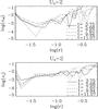 |
Fig. 7 Values of α2D (obtained by averaging all quantities along the z-axis) and αz (the difference of α and α2D representing the contribution of the fluctuations along z) for run ASR2h. The two quantities have comparable values in the inner part of the disc. |
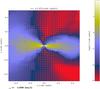 |
Fig. 8 Density and velocity field in the xz plane of the simulation ASR2. Accretion also proceeds from above and below the disc plane along the z-axis. |
Structures along the z-axis apparently play a role in producing somewhat higher values of α, therefore Fig. 8 displays the density and velocity fields in the xz plane for the ASR2h simulations. The result is as expected: a significant velocity field is seen in the z-direction, and the shape of the disc appears to be irregular and not symmetric. This latter point is probably at the origin of the observed difference. In 3D, the gas can enter through the disc directly from above and below instead of only inflowing inside the equatorial plane, as in 2D. This certainly produces a higher accretion rate, but is also likely to generate more turbulence through accretion since gas that approaches the disc from above undergoes a violent gravitational acceleration along the z-axis and shocks. This infall process most likely drives further turbulence.
This could indicate that 2D simulations may generically underestimate the accretion-driven turbulence process in accretion discs. Unless the gas temperature varies abruptly inside the disc, the scale height of the accreting gas must be at least equal to that of the disc at its outer edge. Because the accreting gas is expected to fall onto the disc supersonically, it seems clear that even when it approaches the disc close to the equatorial plane, it will not pile up at the outer disc radius, but will probably reach smaller radii from above (bottom).
5. Influence of symmetry and angular momentum
In this last section we briefly explore the impact of other aspects of the accretion flow, namely its symmetry and its angular momentum. It is important to remember that the exact way in which accretion proceeds is not well known because it depends on the whole history of the star formation process. Previous 2D simulations carried out in Lesur et al. (2015) have shown that the accretion rate is not the only parameter to have a significant influence on the disc.
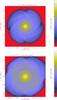 |
Fig. 9 Simulation SR2 (symmetrical accretion with U0 = 2). Column density map at two different time steps. |
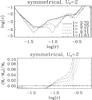 |
Fig. 10 Symmetrical accretion rate with U0 = 2. α values and cumulated mass difference as a function of radius, r. |
5.1. Axisymmetric case
Figure 9 shows the column density at two different time steps for simulation SR2. It clearly appears that the dominant mode is not m = 1, as is the case for ASR2. Instead, m = 4 has developed and become dominant. We note that Cartesian coordinates are probably responsible for the excitation of the m = 4 mode. In the 2D axisymmetric simulations presented in Lesur et al. (2015), the m = 4 mode did not dominate. The spiral wave is tightly wound in the inner part of the disc and more open in the outer part. We recall that Hennebelle et al. (2016) showed that the mass and angular momentum fluxes are higher for smaller m. This is a simple consequence of the disc being more axisymmetric for high m.
The α value and the cumulative mass distribution are shown in Fig. 10. They are to be compared with simulation ASR2, which has the same resolution (left panel of Fig. 4). It appears that while the α values are comparable in the outer part of the disc (log r ≃ −0.6) to what is obtained for ASR2, they quickly drop in the inner part of the disc and almost reach the floor values inferred from the non-accreting simulation.
This behaviour is in good agreement with the cumulative mass distribution. While it is as high as in ASR2, in the outer part of the disc it quickly drops in the disc inner part, indicating that the mass flux is significantly lower than for ASR2.
5.2. Accretion of non-rotating gas
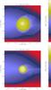 |
Fig. 11 Simulation ASNR2 (asymmetrical accretion with U0 = 2 and no rotation). Column density map at two different time steps. The disc quickly shrinks. |
Finally, since angular momentum is another quantity that plays an important role and its distribution is not well understood, Fig. 11 presents a calculation in which the accreted gas is injected without angular momentum. The impact on the disc is very drastic since its radius shrinks by almost a factor 2. This is because on one hand the centrifugal radius is proportional to j2, j being the specific angular momentum, and on the other hand, the specific angular momentum decreases because the total mass increases, but not the total angular momentum. At the time corresponding to the second snapshot (t = 11.62), the mass in the box has increased by about 40%. Therefore the specific angular momentum has decreased by the same amount, and since 1.42 ≃ 2, we achieve a reasonable agreement. The α values are not been displayed here for conciseness and are also much higher than for the other cases; they typically reach around 0.1. Interestingly, although the disc dynamics appears to be rather vigorous, there are no signs of the prominent spiral pattern that develops in ASR2 in the vicinity of the disc. As discussed above, this is probably due to the absence of rotation within the accreting gas.
These two cases clearly illustrate that the accretion rate is not the only parameter that plays a role. There is therefore considerable uncertainty, and there may be a broad diversity of situations depending on the real distribution of the accretion episode in star formation regions.
6. Discussion: interpretation of observations
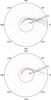 |
Fig. 12 Elliptical orbits for various particles with the same energy, but different trajectories mimicking the accretion studied in this paper (top panel) and particles with different energies (specified by η = r0/rd), but same angular momentum. The orbits clearly tend to approach or even cross each other, which would result in a shock and a spiral arm. |
Many observations of evolved transition discs at various wavelengths from radio to optical have been carried out in recent years (e.g. Hashimoto et al. 2011; Garufi et al. 2013; Boccaletti et al. 2013; Christiaens et al. 2014; Avenhaus et al. 2014; Wagner et al. 2015; Benisty et al. 2015). They consistently reported the presence of density structures such as prominent spiral arms located within or in the vicinity of the disc. The origin of these structures remains debated. They have often been attributed to the presence of a massive planet, which might indeed excite spiral patterns (e.g. Rafikov 2002; Baruteau et al. 2014). Self-gravity is another mechanism that has been proposed to explain these waves, but it is not quite clear whether all the discs with spiral patterns are massive enough (see discussion in Hall et al. 2016).
While these explanations are certainly possible, the simulations performed in this work suggest that accretion is another viable mechanism. Indeed, visual inspection and comparison between Fig. 3 and figures such as Fig. 1 of Hashimoto et al. (2011) or Fig. 1 of Benisty et al. (2015) show a striking resemblance with clear spiral patterns that tend to open up as they retreat from the disc. In the simulation at least, these spiral features are clearly a consequence of the accretion of rotating gas that approaches centrifugal equilibrium (we recall that these spiral arms are absent in the non-rotating accretion case shown in Fig. 11). To understand this more quantitatively, we follow a rotating fluid particle that is infalling toward a star. We assume that its specific angular momentum, j, is conserved, and we ignore all forces except for gravity and centrifugal acceleration. Angular momentum conservation and energy conservation lead to 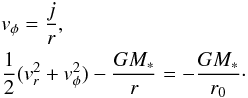 (16)By combining them, we can express
 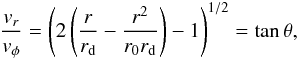 (17)where rd = j2/GM∗ is the centrifugal radius and θ is the angle between the stream line and the azimuthal direction. We stress that the trajectories are Keplerian orbits of various eccentricity. Figure 12 shows five orbits corresponding to the same angular momentum and energy, but different trajectories, mimicking the accretion used in the simulations we presented here (upper panel), and five orbits with different energies (leading to different values of r0 = ηrd, where rd is the Keplerian radius and corresponds to the blue circle), which would result from energy dissipation in the accretion flow (lower panels). The five values of η are 1, 2.1, 2.6, 3.1, and 3.6. Interestingly, the orbits approach very closely to each other and even cross, which would unavoidably result in a shock and a spiral structure. It is tempting to attribute the formation of the prominent spiral structures seen in Fig. 3 to this mechanism. These spirals could therefore be nearly kinematic waves (Toomre 1977).
From Eq. (17), we see that the stream line typically makes an angle θ ≃ 45° just before it enters the disc. This angle increases at larger radii, and is about 60° at r = 2rd, for example. We note that if energy is not conserved, which is likely the case close to the disc because of the shock, then the angle θ is accordingly reduced. Moreover, we stress that the disc radius is not so well determined, in particular, because the incoming particles impact on its surface (compare Figs. 1 and 3), therefore the spiral arm may be able to penetrate “inside” the disc, as is the case in Fig. 12 and in simulations ASR2.
If this interpretation of the origin of some of the observed spiral pattern is confirmed, this would constitute a signature of ongoing accretion in transitional discs.
7. Conclusion
We have investigated the influence that infall may have onto low-mass circumstellar protoplanetary discs by performing 3D hydrodynamical numerical simulations ignoring self-gravity. The underlying idea here was to concentrate on hydrodynamics to distinguish the effects of the different physical processes.
Our results confirm the 2D simulation results presented in Lesur et al. (2015): infall onto the disc has an influence, even at small radii. For an infall rate inside the computational box of about 4 × 10⁻⁷M⊙ yr-1 (which corresponds to an effective accretion rate onto the disc about three to four times lower), we obtained α values inside the disc (that is, at radii about five times smaller than the disc radius) that are as high as 5 × 10⁻³ when the disc has a mass of the order of 10-2M⊙ and a typical thickness H/R ≃ 0.15. At the disc outer edge, values of α up to 10-1 are obtained. These values decrease with the infall rate, and for 10-7M⊙ yr-1 (corresponding to an infall onto the disc about four times smaller), we obtain α values typically three to five times lower, that is to say, equal to about 10-3.
As these α values are a few times higher than the values that have been measured by Lesur et al. (2015), we have estimated the contribution to α of the vertically averaged flows. The associated stress, α2D, was compared to the quantity αz = α−α2D, which quantifies the transport associated with 3D structures. We found that α2D and αz have similar values in the inner part of the disc. This suggests that 3D dynamical processes, in particular the fact that the accreted gas can fall onto the disc from above and below rather than from the equatorial plane alone, plays a role and produces stronger fluctuations. For the conditions that we explored here, we found that typically about 10% of the mass injected in the computational box is accreted deep inside the disc (at a radius smaller than half its initial radius). Since the mass that effectively falls onto the disc is three to four times lower than the mass injected into the box, the mass that is being accreted in the inner part of the disc is about half the mass that effectively falls onto it, although defining the disc boundary accurately appears to be a difficult task.
Finally, we also explored the influence of the symmetry and the angular momentum of the accreted gas, finding that both have a significant influence on the effects that infall has onto the disc. More symmetrical flows have a more limited influence, while slowly rotating material may influence the disc dramatically since it reduces the specific angular momentum. This clearly indicates that precisely quantifying the impact that infall may have on discs requires a detailed knowledge of the star formation process and the nearby environment of the star-disc system.
The accretion of rotating gas naturally produces prominent spiral patterns both inside and outside the disc. The latter seems to be a natural consequence of spiralling collapsing gas dynamics and mainly triggers the spiral pattern within the disc. This pattern presents a striking resemblance with recent observations of transitional discs, which may indicate that at least some of the spirals observed in these objects are due to infalling motions rather than due to the presence of planets.
Acknowledgments
This work was granted access to HPC resources of CINES under the allocation x2014047023 made by GENCI (Grand Équipement National de Calcul Intensif). This research has received funding from the European Research Council under the European Community’s Seventh Framework Programme (FP7/2007-2013 Grant Agreement No. 306483).
References
- Armitage, P. J. 2011, ARA&A, 49, 195 [NASA ADS] [CrossRef] [EDP Sciences] [Google Scholar]
- Avenhaus, H., Quanz, S. P., Schmid, H. M., et al. 2014, ApJ, 781, 87 [NASA ADS] [CrossRef] [Google Scholar]
- Balbus, S. A. 2003, ARA&A, 41, 555 [NASA ADS] [CrossRef] [Google Scholar]
- Baruteau, C., Crida, A., Paardekooper, S.-J., et al. 2014, Protostars and Planets VI, 667 [Google Scholar]
- Benisty, M., Juhasz, A., Boccaletti, A., et al. 2015, A&A, 578, L6 [NASA ADS] [CrossRef] [EDP Sciences] [Google Scholar]
- Boccaletti, A., Pantin, E., Lagrange, A.-M., et al. 2013, A&A, 560, A20 [NASA ADS] [CrossRef] [EDP Sciences] [Google Scholar]
- Christiaens, V., Casassus, S., Perez, S., van der Plas, G., & Ménard, F. 2014, ApJ, 785, L12 [Google Scholar]
- D’Alessio, P., Cantö, J., Calvet, N., & Lizano, S. 1998, ApJ, 500, 411 [NASA ADS] [CrossRef] [Google Scholar]
- Garufi, A., Quanz, S. P., Avenhaus, H., et al. 2013, A&A, 560, A105 [NASA ADS] [CrossRef] [EDP Sciences] [Google Scholar]
- Hall, C., Forgan, D., Rice, K., et al. 2016, MNRAS, 458, 306 [Google Scholar]
- Hashimoto, J., Tamura, M., Muto, T., et al. 2011, ApJ, 729, L17 [NASA ADS] [CrossRef] [Google Scholar]
- Hennebelle, P., Lesur, G., & Fromang, S. 2016, A&A, 590, A22 [NASA ADS] [CrossRef] [EDP Sciences] [Google Scholar]
- Joos, M., Hennebelle, P., & Ciardi, A. 2012, A&A, 543, A128 [NASA ADS] [CrossRef] [EDP Sciences] [Google Scholar]
- Ju, W., Stone, J. M., & Zhu, Z. 2016, ApJ, 823, 81 [NASA ADS] [CrossRef] [Google Scholar]
- Larson, R. B. 1990, MNRAS, 243, 588 [NASA ADS] [Google Scholar]
- Lesur, G., Kunz, M. W., & Fromang, S. 2014, A&A, 566, A56 [NASA ADS] [CrossRef] [EDP Sciences] [Google Scholar]
- Lesur, G., Hennebelle, P., & Fromang, S. 2015, A&A, 582, L9 [NASA ADS] [CrossRef] [EDP Sciences] [Google Scholar]
- Li, Z.-Y., Krasnopolsky, R., & Shang, H. 2013, ApJ, 774, 82 [NASA ADS] [CrossRef] [Google Scholar]
- Lodato, G., & Rice, W. K. M. 2004, MNRAS, 351, 630 [Google Scholar]
- Machida, M. N., Inutsuka, S.-I., & Matsumoto, T. 2010, ApJ, 724, 1006 [NASA ADS] [CrossRef] [Google Scholar]
- Masson, J., Chabrier, G., Hennebelle, P., Vaytet, N., & Commerçon, B. 2016, A&A, 587, A32 [NASA ADS] [CrossRef] [EDP Sciences] [Google Scholar]
- Muzerolle, J., Luhman, K. L., Briceño, C., Hartmann, L., & Calvet, N. 2005, ApJ, 625, 906 [NASA ADS] [CrossRef] [Google Scholar]
- Rafikov, R. R. 2002, ApJ, 569, 997 [NASA ADS] [CrossRef] [Google Scholar]
- Rozyczka, M., & Spruit, H. C. 1993, ApJ, 417, 677 [NASA ADS] [CrossRef] [Google Scholar]
- Sawada, K., Matsuda, T., Inoue, M., & Hachisu, I. 1987, MNRAS, 224, 307 [NASA ADS] [CrossRef] [Google Scholar]
- Spruit, H. C. 1987, A&A, 184, 173 [NASA ADS] [Google Scholar]
- Spruit, H. C., Matsuda, T., Inoue, M., & Sawada, K. 1987, MNRAS, 229, 517 [NASA ADS] [CrossRef] [Google Scholar]
- Teyssier, R. 2002, A&A, 385, 337 [NASA ADS] [CrossRef] [EDP Sciences] [Google Scholar]
- Toomre, A. 1977, ARA&A, 15, 437 [CrossRef] [Google Scholar]
- Turner, N. J., Fromang, S., Gammie, C., et al. 2014, Protostars and Planets VI, 411 [Google Scholar]
- Vishniac, E. T., & Diamond, P. 1989, ApJ, 347, 435 [NASA ADS] [CrossRef] [Google Scholar]
- Vorobyov, E. I., & Basu, S. 2008, ApJ, 676, L139 [NASA ADS] [CrossRef] [Google Scholar]
- Vorobyov, E. I., Lin, D. N. C., & Guedel, M. 2015, A&A, 573, A5 [NASA ADS] [CrossRef] [EDP Sciences] [Google Scholar]
- Wagner, K., Apai, D., Kasper, M., & Robberto, M. 2015, ApJ, 813, L2 [NASA ADS] [CrossRef] [Google Scholar]
- Yukawa, H., Boffin, H. M. J., & Matsuda, T. 1997, MNRAS, 292, 321 [NASA ADS] [CrossRef] [Google Scholar]
All Tables
All Figures
|
Fig. 1 Case of no accretion. Column density map. The disc has a radius of about r = 0.25. |
| In the text | |
|
Fig. 2 Case of no accretion. Column density (top panel) and α value (bottom panel) as a function of the radius r. Typical variations remains limited, and the α values are below 10-3 and rapidly fall below 3 × 10⁻⁴. Note that at small radii (log (r) < −1.6), α increases to high values because of the low resolution. |
| In the text | |
|
Fig. 3 Simulation ASR2 (asymmetrical accretion with U0 = 2 and standard resolution, left panels) and ASR2h (high resolution, right panels). Column density map at three different time steps. The disc initially has a radius of about r = 0.25. Note that the spiral pattern is remarkably stationary. |
| In the text | |
|
Fig. 4 Simulations ASR2 (left) and ASR2h (right). Top panels: α as a function of the radius r. Bottom panels: cumulated mass difference over total mass (see text). Solid lines at r = 0.25 represent the initial disc edge. |
| In the text | |
|
Fig. 5 Azimuthal profiles from simulation ASR2h at time t = 0.75 and at radius r = 0.08 (solid line), 0.14 (dotted), and 0.18 (dashed). Note that the density and the azimuthal velocity have been normalised such that their peak value is equal to 1. |
| In the text | |
|
Fig. 6 Simulations ASR0.5h. α values and cumulated mass difference as a function of radius, r. |
| In the text | |
|
Fig. 7 Values of α2D (obtained by averaging all quantities along the z-axis) and αz (the difference of α and α2D representing the contribution of the fluctuations along z) for run ASR2h. The two quantities have comparable values in the inner part of the disc. |
| In the text | |
|
Fig. 8 Density and velocity field in the xz plane of the simulation ASR2. Accretion also proceeds from above and below the disc plane along the z-axis. |
| In the text | |
|
Fig. 9 Simulation SR2 (symmetrical accretion with U0 = 2). Column density map at two different time steps. |
| In the text | |
|
Fig. 10 Symmetrical accretion rate with U0 = 2. α values and cumulated mass difference as a function of radius, r. |
| In the text | |
|
Fig. 11 Simulation ASNR2 (asymmetrical accretion with U0 = 2 and no rotation). Column density map at two different time steps. The disc quickly shrinks. |
| In the text | |
|
Fig. 12 Elliptical orbits for various particles with the same energy, but different trajectories mimicking the accretion studied in this paper (top panel) and particles with different energies (specified by η = r0/rd), but same angular momentum. The orbits clearly tend to approach or even cross each other, which would result in a shock and a spiral arm. |
| In the text | |
Current usage metrics show cumulative count of Article Views (full-text article views including HTML views, PDF and ePub downloads, according to the available data) and Abstracts Views on Vision4Press platform.
Data correspond to usage on the plateform after 2015. The current usage metrics is available 48-96 hours after online publication and is updated daily on week days.
Initial download of the metrics may take a while.