| Issue |
A&A
Volume 603, July 2017
|
|
|---|---|---|
| Article Number | C2 | |
| Number of page(s) | 6 | |
| Section | The Sun | |
| DOI | https://doi.org/10.1051/0004-6361/201629122e | |
| Published online | 03 July 2017 | |
The global distribution of magnetic helicity in the solar corona (Corrigendum)⋆
1 Department of Mathematical Sciences, Durham University, Durham, DH1 3LE, UK
e-mail: This email address is being protected from spambots. You need JavaScript enabled to view it.
2 Division of Mathematics, University of Dundee, Dundee, DD1 4HN, UK
Key words: magnetic fields / magnetohydrodynamics (MHD) / Sun: corona / Sun: magnetic fields / Sun: coronal mass ejections (CMEs) / errata, addenda
Movies associated to Figs. 10 and 12 are available at http://www.aanda.org
It has come to our attention that incorrect units were inadvertently used for the axes and colour scales of a number of figures in our paper (Yeates & Hornig 2016). Specifically:
-
1.
The units of field line helicity
 are quoted asMaxwells [Mx], but the values for shown inFigs. 3, 5, 7, 10, 11e and 12 in theoriginal paper were actually in
  . They should be multiplied by (6.96 × 10¹⁰)2 toreach the true value in Mx.
 -
2.
The units of total helicity H, and of dH/ dt are quoted as Mx2, but the values were actually in
 . This applies to Figs. 4c, d, 8c, d and 11d. They should be multiplied by (6.96 × 10¹⁰)4 to reach the true value in Mx2.
Corrected versions of the affected figures are included here. This does not in any way affect the qualitative results or conclusions of the paper, but we would like to correct the error for the benefit
of future readers who may wish to make quantitative comparisons.
To put the corrected values into context, DeVore (2000) estimates that the typical helicity content of a single interplanetary magnetic cloud is of the order 2 × 1042 Mx2, which is similar to that shed in our axisymmetric flux rope (Fig. 8c). And Berger & Ruzmaikin (2000) estimate a net transfer rate of helicity due to solar rotation of up to 5 × 1043 Mx day-1 in each hemisphere, at solar maximum. This is also consistent with our results, although a more detailed comparison with a fully data-driven simulation remains to be performed in the future.
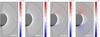 |
Fig. 3 Illustration of the dipolar simulation with ν0 = 0.36 × 10⁻⁵ s-1 on days 0, 1, 2, and 20. Greyscale shading on r = r0 shows Br (white positive, black negative, saturated at ± 0.5 G), and projected coronal magnetic field lines traced from height r = R⊙ are coloured (red/blue) according to |

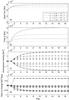 |
Fig. 4 Various integrated quantities as a function of time, for the dipolar simulations with different ν0 (indicated by line styles). Panel a) shows the open magnetic flux ∫r = r1 | Br | dΩ, panel b) shows ∫D | j | dV, and panel c) shows HN (asterisks) and HS (circles). Panel d) shows the terms in Eq. (18) for the northern hemisphere, with asterisks denoting S0, circles S1, squares Seq, and diamonds SV. |
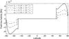 |
Fig. 5 Latitudinal distribution of field line helicity for the dipolar simulations, showing how the peak value tends to zero as the friction parameter ν0 is successively doubled. A log-log fit shows that |

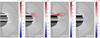 |
Fig. 7 Illustration of the quadrupolar simulation with ν0 = 0.36 × 10⁻⁵ s-1 on days 0, 20, 66, and 68. Greyscale shading on r = r0 shows Br (white positive, black negative, saturated at ± 2 G), and projected coronal magnetic field lines traced from height r = 1.2R⊙ are coloured (red/blue) according to |
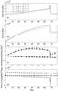 |
Fig. 8 Various integrated quantities as a function of time, for the quadrupolar simulations with different ν0 (indicated by line styles). The format is the same as Fig. 4. For clarity, panel d) shows only the run with ν0 = 0.36 × 10⁻⁵ s-1, and only for the northern hemisphere, although the hemispheres are no longer symmetric. The peak value of S1 during the flux rope eruption is not shown, and is much larger, about − 2.7 × 1043 Mx2 day-1. |
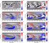 |
Fig. 10 Projected magnetic field lines in the period A (left column) and B (right column) simulations, on days 0, 60, 120, and 180. Greyscale shading on r = r0 shows Br (white positive, black negative, saturated at ± 10 G), and projected coronal magnetic field lines traced from height r = r0 are coloured (red/blue) according to |
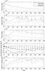 |
Fig. 11 Various integrated quantities as a function of time, for the non-axisymmetric simulations (periods A and B). Panel a) shows the total photospheric magnetic flux ∫r = r0 | Br | dΩ, panel b) shows the total open flux ∫r = r1 | Br | dΩ, panel c) shows ∫D | j | dV, panel d) shows HN (asterisks) and HS (circles), and panel e) shows the root-mean-square field line helicity |
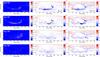 |
Fig. 12 Example of a flux rope ejection from period A. From top to bottom, the rows show days 122, 124, 126, and 128. The left column shows the (absolute) running daily difference of horizontal field |

Movies
Movie 1 of Fig. 10 Access Supplementary Material
Movie 2 of Fig. 10 Access Supplementary Material
Movie 1 of Fig. 12 Access Supplementary Material
Movie 2 of Fig. 12 Access Supplementary Material
References
- Berger, M. A., & Ruzmaikin, A. 2000, J. Geophys. Res., 105, 10481 [NASA ADS] [CrossRef] [Google Scholar]
- DeVore, C. R. 2000, ApJ, 539, 944 [NASA ADS] [CrossRef] [Google Scholar]
- Yeates, A. R., & Hornig, G. 2016, A&A, 594, A98 [NASA ADS] [CrossRef] [EDP Sciences] [Google Scholar]
© ESO, 2017
All Figures
|
Fig. 3 Illustration of the dipolar simulation with ν0 = 0.36 × 10⁻⁵ s-1 on days 0, 1, 2, and 20. Greyscale shading on r = r0 shows Br (white positive, black negative, saturated at ± 0.5 G), and projected coronal magnetic field lines traced from height r = R⊙ are coloured (red/blue) according to |
| In the text | |
|
Fig. 4 Various integrated quantities as a function of time, for the dipolar simulations with different ν0 (indicated by line styles). Panel a) shows the open magnetic flux ∫r = r1 | Br | dΩ, panel b) shows ∫D | j | dV, and panel c) shows HN (asterisks) and HS (circles). Panel d) shows the terms in Eq. (18) for the northern hemisphere, with asterisks denoting S0, circles S1, squares Seq, and diamonds SV. |
| In the text | |
|
Fig. 5 Latitudinal distribution of field line helicity for the dipolar simulations, showing how the peak value tends to zero as the friction parameter ν0 is successively doubled. A log-log fit shows that |
| In the text | |
|
Fig. 7 Illustration of the quadrupolar simulation with ν0 = 0.36 × 10⁻⁵ s-1 on days 0, 20, 66, and 68. Greyscale shading on r = r0 shows Br (white positive, black negative, saturated at ± 2 G), and projected coronal magnetic field lines traced from height r = 1.2R⊙ are coloured (red/blue) according to |
| In the text | |
|
Fig. 8 Various integrated quantities as a function of time, for the quadrupolar simulations with different ν0 (indicated by line styles). The format is the same as Fig. 4. For clarity, panel d) shows only the run with ν0 = 0.36 × 10⁻⁵ s-1, and only for the northern hemisphere, although the hemispheres are no longer symmetric. The peak value of S1 during the flux rope eruption is not shown, and is much larger, about − 2.7 × 1043 Mx2 day-1. |
| In the text | |
|
Fig. 10 Projected magnetic field lines in the period A (left column) and B (right column) simulations, on days 0, 60, 120, and 180. Greyscale shading on r = r0 shows Br (white positive, black negative, saturated at ± 10 G), and projected coronal magnetic field lines traced from height r = r0 are coloured (red/blue) according to |
| In the text | |
|
Fig. 11 Various integrated quantities as a function of time, for the non-axisymmetric simulations (periods A and B). Panel a) shows the total photospheric magnetic flux ∫r = r0 | Br | dΩ, panel b) shows the total open flux ∫r = r1 | Br | dΩ, panel c) shows ∫D | j | dV, panel d) shows HN (asterisks) and HS (circles), and panel e) shows the root-mean-square field line helicity |
| In the text | |
|
Fig. 12 Example of a flux rope ejection from period A. From top to bottom, the rows show days 122, 124, 126, and 128. The left column shows the (absolute) running daily difference of horizontal field |
| In the text | |
Current usage metrics show cumulative count of Article Views (full-text article views including HTML views, PDF and ePub downloads, according to the available data) and Abstracts Views on Vision4Press platform.
Data correspond to usage on the plateform after 2015. The current usage metrics is available 48-96 hours after online publication and is updated daily on week days.
Initial download of the metrics may take a while.