| Issue |
A&A
Volume 581, September 2015
|
|
|---|---|---|
| Article Number | L3 | |
| Number of page(s) | 5 | |
| Section | Letters | |
| DOI | https://doi.org/10.1051/0004-6361/201526626 | |
| Published online | 07 September 2015 | |
VLT/SPHERE- and ALMA-based shape reconstruction of asteroid (3) Juno ⋆
1 Department of Mathematics, Tampere University of Technology, PO Box 553, 33101 Tampere, Finland
e-mail: matti.viikinkoski@tut.fi
2 Astronomical Institute, Faculty of Mathematics and Physics, Charles University in Prague, V Holešovičkách 2, 18000 Prague, Czech Republic
3 ACME, IMCCE, UMR 8028 du CNRS, UPMC, Université de Lille 1, 77 Av. Denfert-Rochereau, 75014 Paris, France
4 Laboratoire Lagrange, UMR 7293 CNRS, UNS, Observatoire de la Côte d’Azur, 06304 Nice, France
5 European Southern Observatory (ESO), Alonso de Còrdova 3107, 1900 Casilla Vitacura, Santiago, Chile
6 Aix-Marseille University, CNRS, LAM (Laboratoire d’Astrophysique de Marseille) UMR 7326, 13388 Marseille, France
7 ONERA − Optics Department, 29 avenue de la Division Leclerc, 92322 Chatillon Cedex, France
8 Southwest Research Institute, 1050 Walnut St., #300 Boulder, CO 80302, USA
9 Unidad Mixta Internacional FCA (UMI 3386), CNRS/INSU & Universidad de Chile, Las Condes, Santiago, Chile
10 LESIA (UMR 8109), Observatoire de Paris, CNRS, UPMC, Univ. Paris-Diderot, PSL, 5 place Jules Janssen, 92195 Meudon, France
Received: 28 May 2015
Accepted: 12 August 2015
We use the recently released Atacama Large Millimeter Array (ALMA) and VLT/SPHERE science verification data, together with earlier adaptive-optics images, stellar occultation, and lightcurve data to model the 3D shape and spin of the large asteroid (3) Juno with the all-data asteroid modelling (ADAM) procedure. These data set limits on the plausible range of shape models, yielding reconstructions suggesting that, despite its large size, Juno has sizable unrounded features moulded by non-gravitational processes such as impacts.
Key words: instrumentation: interferometers / instrumentation: adaptive optics / methods: numerical / minor planets, asteroids: individual: (3) Juno
Based on observations collected at the European Southern Observatory, Paranal, Chile (prog. ID: 60.A-9379, 086.C-0785), and at the W. M. Keck Observatory, which is operated as a scientific partnership among the California Institute of Technology, the University of California and the National Aeronautics and Space Administration. The Observatory was made possible by the generous financial support of the W.M. Keck Foundation.
© ESO, 2015
1. Introduction
Despite a few early adaptive-optics images suggesting an intriguing shape (Baliunas et al. 2003), the asteroid (3) Juno remains relatively unobserved. The release of the ALMA science verification data1 of Juno (ALMA Partnership et al. 2015) allows us, for the first time, to explore the viability of the shape reconstruction of asteroids from disk-resolved thermal infrared observations. We also use other data to test methods and procedures that employ a wide spectrum of various data sources. In particular, we use the science verification data from SPHERE, the recently commissioned extreme adaptive-optics (AO) system (Beuzit et al. 2008) mounted at the European Southern Observatory (ESO) Very Large Telescope (VLT). We survey the available observations of Juno that can be used for shape reconstruction using the recently introduced modeling (ADAM) package (Viikinkoski et al. 2015) and present a model based on ALMA data, lightcurves, AO images, and stellar occultations.
We discuss the reliability of the reconstruction by using different shape representations and data subsets. We show that all plausible shape-model variations are quite similar and suggest that, despite its large diameter of about 250 km, Juno has sizable unrounded and non-equilibrium features. This is in contrast to the very rounded shapes of the largest asteroids (1) Ceres, (2) Pallas, and (4) Vesta witnessed by the Dawn mission (Russell et al. 2012) or imaged from the ground and Hubble Space Telescope (Thomas et al. 2005; Carry et al. 2008, 2010a), but typical of large asteroids that present large flat facets or concavities as do (21) Lutetia, (52) Europa, or (511) Davida (Conrad et al. 2007; Carry et al. 2010b; Merline et al. 2013).
2. Data modes
2.1. Submillimeter interferometry
Juno was observed with ALMA on 2014 Oct. 19 using between 27 and 33 antennas, thereby providing projected baselines between 26 m and 13 km. At the observed frequencies of 224, 226, 240, and 242 GHz, this corresponds to angular resolutions as high as 0.021′′, or about 30 km projected at the distance of Juno. A total of ten different epochs spread over 4.4 h were acquired, and they correspond to about 60% of its rotation period, each epoch having several hundreds of thousands points in the visibility function plane. As stated by ALMA Partnership et al. (2015), each epoch on Juno lasted for 18 min, during which time Juno rotated 15°. The smearing effect is, however, limited to about 21 mas.
The ALMA data are samples of the Fourier transform (FT) of sky brightness. Unlike most other ALMA users, we can use the raw FT data directly for reconstruction. The “clean” ALMA images obtained by various deconvolution and self-calibration processes inevitably lose and distort some of the original information. On the other hand, there usually are residual antenna-based phase errors in the raw ALMA data (Hezaveh et al. 2013). We discuss the effect of this in Sect. 4.
2.2. Adaptive-optics images
The first adaptive-optics images of Juno were obtained at Mt. Wilson observatory in the 1990s with the 100-inch telescope fitted with the ADOPT adaptive-optics system, providing an angular resolution of 0.080′′ at 800 nm. These observations are documented in Baliunas et al. (2003). The original data were no longer available in a usable format, so we used the images directly from the paper. The image scale in the paper was unknown, so we included it in the optimization as a free parameter.
In 2001 and 2010, we also acquired near-infrared disk-resolved images of Juno with the first-generation AO cameras NIRC2 (Wizinowich et al. 2000; van Dam et al. 2004) on the W. M. Keck II telescope and NACO (Lenzen et al. 2003; Rousset et al. 2003) on the ESO VLT. The angular resolution of these data is of 0.045 and 0.055′′, respectively.
We also present here data we obtained during the science verification2 of the recently commissioned second-generation SPHERE AO system, mounted at the VLT (Beuzit et al. 2008). SPHERE is an instrument designed for exoplanet detection and characterization by high-angular and high-contrast imaging and spectro-imaging. The AO module (Fusco et al. 2006) was therefore designed to provide extremely high fidelity correction, but limited to very bright targets (R ~ 11). We used the classical imaging mode of SPHERE (IRDIS, Dohlen et al. 2008) to image the apparent disk of Juno. The different data sets and observation times are summarized in Table 1. Although the images of Juno obtained with NACO and SPHERE theoretically have the same angular resolution, since they were taken at the same wavelength with the same aperture, the higher Strehl ratio achieved by the latter provides more detailed images (Fig. 4).
Range to observer (Δ, in au) and longitude (λ) and latitude (β) of the sub-Earth point (SEP) of the adaptive-optics images used for the shape reconstruction.
2.3. Optical lightcurves
It has been shown (Kaasalainen et al. 2001) that a three-dimensional convex model can be reconstructed with lightcurves from various observation geometries. However, recovering non-convex features reliably is seldom possible with lightcurves alone (Ďurech & Kaasalainen 2003). On the other hand, lightcurves are crucial for enabling and completing the reconstruction when only a few disk-resolved observations are available (Viikinkoski & Kaasalainen 2014; Viikinkoski et al. 2015). For Juno, 37 relative-magnitude lightcurves were obtained in the years 1954–1991. They are available in an electronic format in the Asteroid Photometric Catalogue3 or in the Database of Asteroid Models from Inversion Techniques (DAMIT)4 (Ďurech et al. 2010). Compared to the recent SPHERE and ALMA observations, even the latest lightcurve is more than 20 years old. Therefore, we acquired a lightcurve in April 2015 at the 1 m telescope of the Pic-du-Midi Observatory, France.
2.4. Stellar occultation
There are six stellar occultation events listed by Dunham et al. (2014) and publicly available on the Planetary Data System (PDS)5. However, only the occultation from 1979 with 16 full chords can be used for recovering an almost complete silhouette, although its timings are not as accurate as is customary nowadays. Ďurech et al. (2011) used this dataset to scale the convex model of Juno reconstructed from lightcurves by Kaasalainen et al. (2002).
3. Methods
We used the ADAM algorithm (Viikinkoski & Kaasalainen 2014; Viikinkoski et al. 2015) for the shape and spin reconstruction. ADAM enables an easy combining and weighting of various data types. In the case of Juno, the ALMA visibility data were combined with disk-integrated photometry and with the adaptive-optics images, and checked against the occultation data. The last did not improve the reliability of the solution or provide more information, so we only used them as a consistency check as depicted in Fig. 5.
Not all the apparent features present in the Mt. Wilson data could be accommodated in any acceptable solution (as defined in Kaasalainen 2011; Kaasalainen & Viikinkoski 2012) based on all the data. This is probably due to non-corrected aberrations by the early AO equipment and/or artifacts introduced by the deconvolution. Indeed, unlike Mistral (Mugnier et al. 2004), the algorithm we used to deconvolve the images from NACO, NIRC2, and SPHERE, the Lucy-Richardson deconvolution of Baliunas et al. (2003) is not optimized for objects with sharp boundaries.
We used both subdivision surfaces and octantoid parametrization for shape representations (Viikinkoski et al. 2015). Based on a global parametrization by spherical harmonics, octantoids produce smooth curved surfaces, while the subdivision surfaces, together with the regularization we use, are characterized by sharper local features. By using two different shape supports, we strove to distinguish the model features caused by the shape representation from those actually supported by the data. Similarly, we checked the effect of data sources by observing the model variations under varying data subset combinations.
For thermal modeling, we used a simple, semi-analytical FFT-based approach (Nesvorný & Vokrouhlický 2008; Viikinkoski & Kaasalainen 2014). While it lacks the sophistication of more detailed models, it is fast and sufficient for recovering the model boundaries, which are the most important feature for shape reconstruction. Also, owing to the very low thermal inertia of Juno of 5 J m-2 s-0.5 K-1 (Mueller & Lagerros 1998), the differences between our approach and more complex ones are expected to remain small.
4. Results
Most of the disk-resolved data (especially those from ALMA and SPHERE) were obtained at viewing geometries restricted to Juno’s southern hemisphere, so the northern parts of the model are less constrained. Figure 3 shows ALMA deconvolved images vs. the ALMA-dominated shape model on the plane of sky. This is not the actual data fit, but a visual aid for illustration purposes. We used the calibrated visibility data instead of the ALMA deconvolved images (that are formed by a strongly iterative separate process and additional assumptions) in the primary reconstruction, and the model images are given as visible wavelength projections that look essentially the same as the thermal ones due to the low thermal inertia. ALMA-dominated models are shown in the first two rows of Fig. 1. These already emphasize the lopsided or lozenge-like shape hinted at by the lightcurve-only model of Kaasalainen et al. (2002). The viewing direction of the Mt. Wilson AO image is almost in the equatorial plane of the asteroid and, despite its lower reliability, provides useful additional information not present in the thermal data.
The model obtained from the full dataset is depicted in the last row of Fig. 1. Comparison of the model with optical lightcurves, AO images, ALMA reconstructed images, and stellar occultation are presented in Figs. 2, 4, 3, and 5, respectively. This model can be downloaded at the DAMIT web site.
There are 11 diameter and 23 mass estimates for (3) Juno in the literature (see Appendix), giving an average diameter of 249 ± 7 km and an average mass of 2.68 ± 0.24 × 10¹⁹ kg. Our determination of 249 ± 5 km corresponds exactly to this average diameter. Using this estimate, we find a density of 3.32 ± 0.40 g cm-3. Compared with the grain density of L ordinary chondrites (Consolmagno et al. 2008), this implies a porosity of 7 ± 1% and a null macroporosity of 2 ± 2%, which is consistent with an intact internal structure. As shown in Table 2, the spin determination by Kaasalainen et al. (2002) and Ďurech et al. (2011) agrees very well with the result here, and the study of AO images from Lick observatory by Drummond & Christou (2008) provides an independent confirmation of this spin location. Although the topography of the northern hemisphere is less constrained than the southern latitudes, the vertical dimension seems stable under shape support and data subset variations.
 |
Fig. 1 Plausible variations of reconstruction. Models are from: ALMA and lightcurves – octantoid (top); subdivision surfaces: combined AO (Mt. Wilson), ALMA and lightcurve data (middle); full data set (bottom). Viewing directions are from the positive x-, y-, and z-axes. |
 |
Fig. 2 Examples of the synthetic lightcurves generated with current ADAM shape model and the lightcurve model (LCI) by Kaasalainen et al. (2002) compared with photometric observations on four epochs. Also the phase angle (α) and the duration of observations are displayed. The models are hardly distinguishable. |
 |
Fig. 3 Comparison of the ALMA deconvolved images (top) to the ALMA+lightcurve model (bottom). The scalebar corresponds to 50 km. |
 |
Fig. 4 Adaptive-optics images used for reconstruction (top) and corresponding model views (bottom). See Table 1 for observing conditions and instruments. The scattering law used for the shading exaggerates surface features. |
We also checked the effect of ALMA self-calibration on the quality of shape reconstruction. During self-calibration, the antenna phase errors causing deteriorated image quality are corrected iteratively, alternating between the frequency and the image domain (ALMA Partnership et al. 2015). The model reconstructed from the self-calibrated, deconvolved images instead of the raw data revealed no additional detail, at least for this level of resolution (even when using ALMA data only), so the self-calibration is not a major concern here. The best way to facilitate full high resolution in shape reconstruction from future full-baseline ALMA data is to let the antenna gains be free parameters (Hezaveh et al. 2013), so that the optimization of the shape, spin, and the antenna parameters is done simultaneously. This prevents the introduction of potentially spurious information into the shape solution.
Comparison of different models.
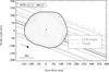 |
Fig. 5 Comparison of the shape model with the chords from the stellar occultation of 1979. The shape model created without the occultation data is very consistent with the occultation chords, although Juno rotated some 13° during the event. |
5. Conclusions
We have reconstructed the shape and spin of (3) Juno from combined thermal interferometry, optical photometry, and adaptive-optics images, and checked its consistency with occultation data. Different and independent shape supports and regularization methods generate similar shapes, suggesting that the main features are actually present in the data, so are not artifacts of the reconstruction. Owing to the restricted observing geometries, the southern hemisphere of Juno is described here better than its northern latitudes. Juno seems to reside in the volumetric and structural transition region from dwarf planets to large and medium-sized asteroids. Its global shape features are apparently molded by other than gravitational processes (likely impacts).
While the angular resolution currently delivered by ALMA is comparable to that of adaptive-optics-fed cameras mounted on 8–10 m telescopes, ALMA will provide a resolution close to 5 mas (Busch 2009) once at full capability. This will convert ALMA into one of the most important sources of disk-resolved asteroid data, alongside adaptive-optics images and range-Doppler radar echoes.
Acknowledgments
This paper makes use of the following ALMA data: ADS/JAO.ALMA#2011.0.00013.SV. ALMA is a partnership of ESO (representing its member states), NSF (USA) and NINS (Japan), together with NRC (Canada) and NSC and ASIAA (Taiwan), in cooperation with the Republic of Chile. The Joint ALMA Observatory is operated by ESO, AUI/NRAO and NAOJ. This research made use of the Keck Observatory Archive (KOA), which is operated by the W. M. Keck Observatory and the NASA Exoplanet Science Institute (NExScI), under contract with the National Aeronautics and Space Administration. The authors wish to recognize and acknowledge the very significant cultural role and reverence that the summit of Mauna Kea has always had within the indigenous Hawaiian community. We are most fortunate to have the opportunity to conduct observations from this mountain. This work was supported by the Centre of Excellence in Inverse Problems Research (Academy of Finland). The work of J.D. was supported by the research grant GACR 15-04816S of the Czech Science Foundation.
References
- ALMA Partnership, Hunter, T. R., Kneissl, R., et al. 2015, ApJ, 808, L2 [NASA ADS] [CrossRef] [Google Scholar]
- Baer, J., Milani, A., Chesley, S. R., & Matson, R. D. 2008, in BAAS, 40, 493 [Google Scholar]
- Baer, J., Chesley, S. R., & Matson, R. D. 2011, AJ, 141, 143 [NASA ADS] [CrossRef] [Google Scholar]
- Baier, G., & Weigelt, G. 1983, A&A, 121, 137 [NASA ADS] [Google Scholar]
- Baliunas, S., Donahue, R., Rampino, M. R., et al. 2003, Icarus, 163, 135 [NASA ADS] [CrossRef] [Google Scholar]
- Barnard, E. E. 1900, MNRAS, 61, 68 [NASA ADS] [CrossRef] [Google Scholar]
- Beuzit, J.-L., Feldt, M., Dohlen, K., et al. 2008, Proc. SPIE, 7014, 701418 [CrossRef] [Google Scholar]
- Busch, M. W. 2009, Icarus, 200, 347 [NASA ADS] [CrossRef] [Google Scholar]
- Carry, B., Dumas, C., Fulchignoni, M., et al. 2008, A&A, 478, 235 [NASA ADS] [CrossRef] [EDP Sciences] [Google Scholar]
- Carry, B., Dumas, C., Kaasalainen, M., et al. 2010a, Icarus, 205, 460 [NASA ADS] [CrossRef] [Google Scholar]
- Carry, B., Kaasalainen, M., Leyrat, C., et al. 2010b, A&A, 523, A94 [NASA ADS] [CrossRef] [EDP Sciences] [Google Scholar]
- Carry, B., Kaasalainen, M., Merline, W. J., et al. 2012, Planet. Space Sci., 66, 200 [Google Scholar]
- Chernetenko, Y. A., & Kochetova, O. M. 2002, in Asteroids, Comets, and Meteors: ACM 2002, ed. B. Warmbein, ESA SP, 500, 437 [Google Scholar]
- Conrad, A. R., Dumas, C., Merline, W. J., et al. 2007, Icarus, 191, 616 [NASA ADS] [CrossRef] [Google Scholar]
- Consolmagno, G., Britt, D., & Macke, R. 2008, Chemie der Erde/Geochemistry, 68, 1 [Google Scholar]
- Dohlen, K., Langlois, M., Saisse, M., et al. 2008, in SPIE Conf. Ser., 7014, 3 [Google Scholar]
- Drummond, J. D., & Christou, J. C. 2008, Icarus, 197, 480 [NASA ADS] [CrossRef] [Google Scholar]
- Dunham, D., Herald, D., Frappa, E., et al. 2014, NASA Planetary Data System, EAR-A-3-RDR-OCCULTATIONS-V12.0 [Google Scholar]
- Ďurech, J., & Kaasalainen, M. 2003, A&A, 404, 709 [NASA ADS] [CrossRef] [EDP Sciences] [Google Scholar]
- Ďurech, J., Sidorin, V., & Kaasalainen, M. 2010, A&A, 513, A46 [NASA ADS] [CrossRef] [EDP Sciences] [Google Scholar]
- Ďurech, J., Kaasalainen, M., Herald, D., et al. 2011, Icarus, 214, 652 [NASA ADS] [CrossRef] [Google Scholar]
- Fienga, A., Manche, H., Kuchynka, P., Laskar, J., & Gastineau, M. 2010, Scientific Notes(INPOP10a) [Google Scholar]
- Fienga, A., Kuchynka, P., Laskar, J., Manche, H., & Gastineau, M. 2011, EPSC-DPS Joint Meeting 2011, 1879 [Google Scholar]
- Fienga, A., Manche, H., Laskar, J., Gastineau, M., & Verma, A. 2013, ArXiv e-prints [arXiv:1301.1510] [Google Scholar]
- Fienga, A., Manche, H., Laskar, J., Gastineau, M., & Verma, A. 2014, ArXiv e-prints [arXiv:1405.0484] [Google Scholar]
- Folkner, W. M., Williams, J. G., & Boggs, D. H. 2009, IPN Progress Report, 42, 1 [Google Scholar]
- Fusco, T., Rousset, G., Sauvage, J.-F., et al. 2006, Optics Express, 14, 7515 [Google Scholar]
- Goffin, E. 2014, A&A, 565, A56 [NASA ADS] [CrossRef] [EDP Sciences] [Google Scholar]
- Hezaveh, Y. D., Marrone, D. P., Fassnacht, C. D., et al. 2013, ApJ, 767, 132 [NASA ADS] [CrossRef] [Google Scholar]
- Kaasalainen, M. 2011, Inverse Problems and Imaging, 5, 37 [CrossRef] [Google Scholar]
- Kaasalainen, M., & Viikinkoski, M. 2012, A&A, 543, A97 [NASA ADS] [CrossRef] [EDP Sciences] [Google Scholar]
- Kaasalainen, M., Torppa, J., & Muinonen, K. 2001, Icarus, 153, 37 [NASA ADS] [CrossRef] [Google Scholar]
- Kaasalainen, M., Torppa, J., & Piironen, J. 2002, Icarus, 159, 369 [NASA ADS] [CrossRef] [Google Scholar]
- Kochetova, O. M. 2004, Solar System Research, 38, 66 [NASA ADS] [CrossRef] [Google Scholar]
- Kochetova, O. M., & Chernetenko, Y. A. 2014, Solar System Research, 48, 295 [NASA ADS] [CrossRef] [Google Scholar]
- Konopliv, A. S., Asmar, S. W., Folkner, W. M., et al. 2011, Icarus, 211, 401 [NASA ADS] [CrossRef] [Google Scholar]
- Konopliv, A. S., Yoder, C. F., Standish, E. M., Yuan, D.-N., & Sjogren, W. L. 2006, Icarus, 182, 23 [NASA ADS] [CrossRef] [Google Scholar]
- Kuchynka, P., & Folkner, W. M. 2013, Icarus, 222, 243 [NASA ADS] [CrossRef] [Google Scholar]
- Lenzen, R., Hartung, M., Brandner, W., et al. 2003, in SPIE Conf. Ser. 4841, eds. M. Iye, & A. F. M. Moorwood, 944 [Google Scholar]
- Masiero, J. R., Mainzer, A. K., Grav, T., et al. 2012, ApJ, 759, L8 [NASA ADS] [CrossRef] [Google Scholar]
- Merline, W. J., Drummond, J. D., Carry, B., et al. 2013, Icarus, 225, 794 [NASA ADS] [CrossRef] [Google Scholar]
- Millis, R. L., Wasserman, L. H., Bowell, E., et al. 1981, AJ, 86, 306 [NASA ADS] [CrossRef] [Google Scholar]
- Morrison, D., & Zellner, B. 2007, TRIAD Radiometric Diameters and Albedos, NASA Planetary Data System, EAR-A-COMPIL-5-TRIADRAD-V1.0 [Google Scholar]
- Mueller, T. G., & Lagerros, J. S. V. 1998, A&A, 338, 340 [NASA ADS] [Google Scholar]
- Mugnier, L. M., Fusco, T., & Conan, J.-M. 2004, J. Opt. Soc. Am. A, 21, 1841 [NASA ADS] [CrossRef] [Google Scholar]
- Nesvorný, D., & Vokrouhlický, D. 2008, AJ, 136, 291 [NASA ADS] [CrossRef] [Google Scholar]
- Pitjeva, E. V. 2004, in COSPAR, Plenary Meeting, Vol. 35, 35th COSPAR Scientific Assembly, ed. J.-P. Paillé, 2014 [Google Scholar]
- Pitjeva, E. V. 2005, Solar System Research, 39, 176 [Google Scholar]
- Pitjeva, E. V. 2010, in IAU Symp. 261, eds. S. A. Klioner, P. K. Seidelmann, & M. H. Soffel, 170 [Google Scholar]
- Pitjeva, E. V. 2013, Solar System Research, 47, 386 [NASA ADS] [CrossRef] [Google Scholar]
- Rousset, G., Lacombe, F., Puget, P., et al. 2003, in SPIE Conf. Ser. 4839, eds. P. L. Wizinowich, & D. Bonaccini, 140 [Google Scholar]
- Russell, C. T., Raymond, C. A., Coradini, A., et al. 2012, Science, 336, 684 [NASA ADS] [CrossRef] [Google Scholar]
- Ryan, E. L., & Woodward, C. E. 2010, AJ, 140, 933 [NASA ADS] [CrossRef] [Google Scholar]
- Somenzi, L., Fienga, A., Laskar, J., & Kuchynka, P. 2010, Planet. Space Sci., 58, 858 [NASA ADS] [CrossRef] [Google Scholar]
- Tedesco, E. F., Noah, P. V., Noah, M. C., & Price, S. D. 2004, IRAS Minor Planet Survey, NASA Planetary Data System, IRAS-A-FPA-3-RDR-IMPS-V6.0 [Google Scholar]
- Thomas, P. C., Parker, J. W., McFadden, L. A., et al. 2005, Nature, 437, 224 [NASA ADS] [CrossRef] [PubMed] [Google Scholar]
- Usui, F., Kuroda, D., Müller, T. G., et al. 2011, Pub. Astron. Soc. Japan, 63, 1117 [CrossRef] [Google Scholar]
- van Dam, M. A., Le Mignant, D., & Macintosh, B. A. 2004, Appl. Opt., 43, 5458 [NASA ADS] [CrossRef] [Google Scholar]
- Viikinkoski, M., & Kaasalainen, M. 2014, Inverse Problems and Imaging, 8, 885 [Google Scholar]
- Viikinkoski, M., Kaasalainen, M., & Ďurech, J. 2015, A&A, 576, A8 [NASA ADS] [CrossRef] [EDP Sciences] [Google Scholar]
- Wizinowich, P. L., Acton, D. S., Lai, O., et al. 2000, in SPIE Conf. Ser. 4007, ed. P. L. Wizinowich, 2 [Google Scholar]
- Zielenbach, W. 2011, AJ, 142, 120 [NASA ADS] [CrossRef] [Google Scholar]
Appendix A: Diameter and mass estimates from the literature
There are 11 diameter estimates of (3) Juno in the literature, obtained with a wide variety of techniques (see Fig. A.1 and Barnard 1900; Morrison & Zellner 2007; Tedesco et al. 2004; Millis et al. 1981; Baier & Weigelt 1983; Drummond & Christou 2008; Ryan & Woodward 2010; Ďurech et al. 2011; Usui et al. 2011; Masiero et al. 2012). We determine the average value here following the method by Carry et al. (2012), by rejecting all the estimates that do not fall within one standard deviation of the average value, then by recomputing the average without these values.
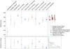 |
Fig. A.1 Diameter estimates of (3) Juno gathered from the literature. The dashed lines depict 3% deviation from the mean. |
Similarly, there are 23 mass estimates for (3) Juno, obtained by studying the orbital deflection of other minor planets (see Fig. A.2 and Chernetenko & Kochetova 2002; Kochetova 2004; Pitjeva 2004, 2005, 2010, 2013; Konopliv et al. 2006, 2011; Baer et al. 2008, 2011; Folkner et al. 2009; Fienga et al. 2010, 2011, 2013, 2014; Somenzi et al. 2010; Zielenbach 2011; Kuchynka & Folkner 2013; Goffin 2014; Kochetova & Chernetenko 2014). Because there is no known satellite of Juno, mass determination relies on these long-range interactions.
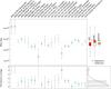 |
Fig. A.2 Mass estimates of (3) Juno gathered from the literature. The dashed lines depict 10% deviation from the mean. |
All Tables
Range to observer (Δ, in au) and longitude (λ) and latitude (β) of the sub-Earth point (SEP) of the adaptive-optics images used for the shape reconstruction.
All Figures
|
Fig. 1 Plausible variations of reconstruction. Models are from: ALMA and lightcurves – octantoid (top); subdivision surfaces: combined AO (Mt. Wilson), ALMA and lightcurve data (middle); full data set (bottom). Viewing directions are from the positive x-, y-, and z-axes. |
| In the text | |
|
Fig. 2 Examples of the synthetic lightcurves generated with current ADAM shape model and the lightcurve model (LCI) by Kaasalainen et al. (2002) compared with photometric observations on four epochs. Also the phase angle (α) and the duration of observations are displayed. The models are hardly distinguishable. |
| In the text | |
|
Fig. 3 Comparison of the ALMA deconvolved images (top) to the ALMA+lightcurve model (bottom). The scalebar corresponds to 50 km. |
| In the text | |
|
Fig. 4 Adaptive-optics images used for reconstruction (top) and corresponding model views (bottom). See Table 1 for observing conditions and instruments. The scattering law used for the shading exaggerates surface features. |
| In the text | |
|
Fig. 5 Comparison of the shape model with the chords from the stellar occultation of 1979. The shape model created without the occultation data is very consistent with the occultation chords, although Juno rotated some 13° during the event. |
| In the text | |
|
Fig. A.1 Diameter estimates of (3) Juno gathered from the literature. The dashed lines depict 3% deviation from the mean. |
| In the text | |
|
Fig. A.2 Mass estimates of (3) Juno gathered from the literature. The dashed lines depict 10% deviation from the mean. |
| In the text | |
Current usage metrics show cumulative count of Article Views (full-text article views including HTML views, PDF and ePub downloads, according to the available data) and Abstracts Views on Vision4Press platform.
Data correspond to usage on the plateform after 2015. The current usage metrics is available 48-96 hours after online publication and is updated daily on week days.
Initial download of the metrics may take a while.