| Issue |
A&A
Volume 553, May 2013
|
|
|---|---|---|
| Article Number | A1 | |
| Number of page(s) | 7 | |
| Section | Astrophysical processes | |
| DOI | https://doi.org/10.1051/0004-6361/201220936 | |
| Published online | 18 April 2013 | |
The thermohaline, Richardson, Rayleigh-Taylor, Solberg–Høiland, and GSF criteria in rotating stars
1
Geneva Observatory, Geneva University, 1290
Sauverny,
Switzerland
e-mail: andre.maeder;This email address is being protected from spambots. You need JavaScript enabled to view it.
; This email address is being protected from spambots. You need JavaScript enabled to view it.
2
School of Physics and Astronomy, University of
Birmingham, Edgbaston, Birmingham
B15 2TT,
UK
e-mail: This email address is being protected from spambots. You need JavaScript enabled to view it.
3
IRAP, CNRS UMR 5277, Univ. de Toulouse, 14 Av. E. Belin,
31400
Toulouse,
France
Received:
17
December
2012
Accepted:
11
March
2013
Abstract
Aims. We examine the interactions of various instabilities in rotating stars, which usually are considered as independent.
Methods. An analytical study of the problem is performed accounting for radiative losses, μ-gradients, and horizontal turbulence.
Results. The diffusion coefficient for an ensemble of instabilities is not given by the sum of the specific coefficients for each instability, but by the solution of a general equation. We find that thermohaline mixing is possible in low-mass red giants only if the horizontal turbulence is very weak. In rotating stars the Rayleigh-Taylor and the shear instabilities need simultaneous treating. This leads to rotation laws of the form 1/rα being predicted to be unstable for α > 1.6568, while the usual Rayleigh criterion only predicts instability for α > 2. Also, the shear instabilities are somehow reduced in main sequence stars by the effect of the Rayleigh-Taylor criterion. Various instability criteria should be expressed differently in rotating stars than in simplified geometries.
Key words: convection / hydrodynamics / instabilities / turbulence
© ESO, 2013
1. Introduction
Various instabilities and processes intervene in stars, particularly in rotating stars, and produce some mixing in radiative zones. These processes are often expressed by diffusion coefficients (Endal & Sofia 1978; Zahn 1992). Currently the global diffusion coefficient is expressed as the sum of the particular coefficients of the various effects considered independently. However, there are many physical interactions between the different instabilities, with possible amplification or damping effects. Our aim here is to consider the interaction of different instabilities and their associated criteria.
The effects and criteria we consider here are the thermohaline instability (Ulrich 1972; Kippenhahn et al. 1980), the shear instability expressed by the Richardson criterion, the Rayleigh-Taylor instability (Chandrasekhar 1961), the semiconvective instability, the instability characterized by the Solberg-Høiland criterion (Wasiutynski 1946), and the baroclinic instability expressed by the Golreich-Schubert-Fricke (GSF) criterion (Goldreich & Schubert 1967; Fricke 1968). We also need to account for nonadiabatic effects, for the μ-gradients, and for the horizontal turbulence generally present in differentially rotating stars. The interactions of horizontal turbulence with shear instabilities and meridional circulation were studied respectively by Talon & Zahn (1997) and by Chaboyer & Zahn (1992). The exact amplitude of the horizontal turbulence is uncertain and various estimates have been performed (Zahn 1992; Maeder 2003; Mathis et al. 2004).
An interesting consequence of this work is that some of the well known instabilities should never be considered alone in rotating stars, but always in their interactions with other ones. This leads to modified expressions of the corresponding criteria when applied to rotating stars.
In Sect. 2, we start by deriving the basic expression of thermohaline mixing in two ways that both show that a proper account of the mean molecular weight is often missing in many derivations. We also analytically examine the effect of the horizontal turbulence on thermohaline mixing. In Sect. 3, we show that many instabilities are interacting and should not be treated separately, but are better analyzed in the frame of a more general equation. In Sect. 4, we reconsider some well known stability criteria and provide new expressions for them in rotating stars. Section 5 gives the conclusions.
2. The double–diffusive mixing revisited
2.1. The thermohaline mixing
We first consider the effects of the gradients of mean molecular weight μ on the stability, since such gradients are always present in stellar interiors as a result of nuclear reactions and ionization. Most of the time the μ-gradients have a stabilizing effect, since regions with higher μ are generally deeper in the star.
The μ-gradient may also be destabilizing, when in a medium subject to gravity some upper layers have a higher mean molecular weight μ than deeper layers (∇μ < 0). The medium may nevertheless be stable with respect to the Ledoux criterion for convection. This is possible, if the upper layers with higher μ are hot enough to allow a stable density gradient. However, if heat diffusion is fast (faster than matter diffusion), the medium of higher μ has the time to cool, become denser, and start sinking. This is the thermohaline instability, which takes the form of “salt fingers” in lab experiments.
The interest for thermohaline mixing has been revived over recent years in relation with the observed chemical abundances of red giants, which require some significant internal mixing at the level of the H-burning shell. Charbonnel & Zahn (2007) and Charbonnel & Lagarde (2010) investigated the effects of thermohaline instability in red giant stars using a classical treatment for the associated diffusion coefficient. They found, in particular, excellent agreement between theoretical predictions and the observations of Li, C, and N isotopes on the upper red giant branch. Also, Lagarde et al. (2012) showed that including thermohaline mixing in stellar models provides a very elegant solution to the longstanding helium-3 problem in the Galaxy. On the other hand, Cantiello & Langer (2010) and Wachlin et al. (2011) have shown that to explain the surface abundances observed at the bump in the luminosity function, the speed of the thermohaline mixing process needs to be some orders of magnitude higher than in their models. These different results are due, at least in large part, to the different geometries adopted for the fluid elements. In these last two works, the fluid elements are essentially spherical, while other authors like Charbonnel & Lagarde (2010) in line with Ulrich (1972) consider elongated “salt fingers”. We see below (Eqs. (3) and (5)) that the ratio of the vertical length of the salt fingers to their diameter intervene to the square as a multiplicative factor in the thermohaline diffusion coefficient.
The theory has been analyzed by Denissenkov & Pinsonneault (2008) in relation to 3He burning in the envelopes of red giants, a work confirmed by 2D numerical simulations (Denissenkov 2010). Further numerical simulations (Denissenkov & Merryfield 2011) suggest that the thermohaline mixing is not efficient enough (by a factor of 50) to account for the observed composition anomalies of red giants. Numerical 3D simulations have been performed by Traxler et al. (2011), who develop new prescriptions and support the inability of thermohaline mixing to achieve the observed mixing, while Brown et al. (2012) find more transport than suggested by Traxler et al. The effect of radiative levitation and turbulence on thermohaline mixing have been nicely analyzed by Vauclair & Théado (2012). On the whole, we see a wide variety of results, often related to the choice of some physical parameters.
2.2. The account of the chemically inhomogeneous surroundings
Often a perturbation method is used to derive the coefficient of thermohaline diffusion
following Ulrich (1972) or a blob method following
Kippenhahn et al. (1980). The problem is that the
possible ambient variations of μ are generally neglected. We consider the
blob method. Kippenhahn et al. (1980) have shown
that the falling velocity vμ of a blob with
an excess Δμ > 0 with respect to the surrounding
medium is given by 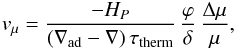 (1)where
τtherm is the thermal adjustment timescale given by
(1)where
τtherm is the thermal adjustment timescale given by
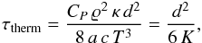 (2)where
K is the thermal diffusivity
K = 4 a c T3/(3 κ ϱ2CP)
and d the diameter of the blob. The factor of 6 applies to a spherical
bubble, while elongated blobs like salt fingers have higher values, e.g. 12, 20, or more.
The usual notations are used, in particular HP the pressure
scale height,
δ = −(∂lnϱ/∂lnT)P,μ,
and
ϕ = (∂lnϱ/∂lnμ)P,T.
In a radiative medium ∇ad > ∇, thus for
Δμ > 0 one has
vμ < 0, and the
blob is sinking.
(2)where
K is the thermal diffusivity
K = 4 a c T3/(3 κ ϱ2CP)
and d the diameter of the blob. The factor of 6 applies to a spherical
bubble, while elongated blobs like salt fingers have higher values, e.g. 12, 20, or more.
The usual notations are used, in particular HP the pressure
scale height,
δ = −(∂lnϱ/∂lnT)P,μ,
and
ϕ = (∂lnϱ/∂lnμ)P,T.
In a radiative medium ∇ad > ∇, thus for
Δμ > 0 one has
vμ < 0, and the
blob is sinking.
The thermohaline diffusion coefficient is
Dthl = |ℓ vμ|
(because the transport is anisotropic, there is no factor 1/3), thus
one has 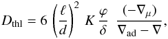 (3)There,
for the expression of the relative excess of mean molecular weight, one generally has
Δμ/μ = ℓ (dlnμ/dr) = −ℓ ∇μ /HP,
where ℓ is the mean free path of the fluid element. The geometrical
factors
6 (ℓ/d)2
can be grouped in a constant Cthl, which may become large for
salt fingers. An expression of the form (3)
was found by Ulrich (1972) with a coefficient
Cthl = 685, and a similar expression, but with
Cthl = 12, was obtained by Kippenhahn et al. (1980). The same expression but with
Cthl = 1000 has been used by Charbonnel & Lagarde (2010), to imply that the mixinglength of the fluid
elements is very large with respect to their diameters. Similar expressions, but with
different coefficients, have also been obtained and used by Denissenkov & Pinsonneault (2008), Théado & Vauclair (2012), and Vauclair
& Théado (2012).
(3)There,
for the expression of the relative excess of mean molecular weight, one generally has
Δμ/μ = ℓ (dlnμ/dr) = −ℓ ∇μ /HP,
where ℓ is the mean free path of the fluid element. The geometrical
factors
6 (ℓ/d)2
can be grouped in a constant Cthl, which may become large for
salt fingers. An expression of the form (3)
was found by Ulrich (1972) with a coefficient
Cthl = 685, and a similar expression, but with
Cthl = 12, was obtained by Kippenhahn et al. (1980). The same expression but with
Cthl = 1000 has been used by Charbonnel & Lagarde (2010), to imply that the mixinglength of the fluid
elements is very large with respect to their diameters. Similar expressions, but with
different coefficients, have also been obtained and used by Denissenkov & Pinsonneault (2008), Théado & Vauclair (2012), and Vauclair
& Théado (2012).
A critical point is that expression (1), hence (3), applies to thermohaline mixing in a surrounding homogeneous medium. This is not the general case, e.g. in a radiative shell H-burning region, there is a μ-gradient throughout the zone where mixing develops. (We may also point out that in the derivation of (3) it is a bit strange to assume the surrounding medium is homogenous and, at the same time, to make use of a certain ∇μ. Maybe, this ∇μ could be considered as the average gradient between the blob and the surrounding medium, but this is not very satisfactory.)
We therefore consider an inhomogeneous medium with a given μ-gradient,
the general form of the sinking velocity vμ
is thus (Maeder 2009), 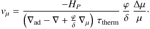 (4)As
a consequence, the thermohaline diffusion coefficient is
(4)As
a consequence, the thermohaline diffusion coefficient is 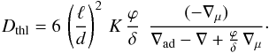 (5)This
expression supports the consistent finding by Denissenkov
(2010) of a term ∇μ at the denominator of (5), a term that is generally ignored, both in
theoretical papers and models of stellar evolution. We examine the size of the various
terms in the numerical model of a 1.25 M⊙ of solar
composition, with an initial rotation velocity of 110 km s-1 at the stage of
the red giant bump with a luminosity of 105 L⊙, as in Fig. 9
by Charbonnel & Lagarde (2010). The zone
where thermohaline mixing is present extends over about 2.6% of the radius around a mass
fraction MR/M = 0.30 at
the base of the extended outer convective zone. Over most of this small zone,
(∇ad − ∇) is around 0.15, while the term
(ϕ/δ) ∇μ
is about 3 × 10⁻⁶, meaning that, even if ∇μ is the
leading term in the numerator its effect on the denominator is negligible here. As a
result the coefficient of thermohaline diffusion is high, lying between 107 and
1010 cm2 s-1, while the coefficients resulting from
other diffusion sources are in the range of 102 to 103
cm2 s-1. So far so good, this would confirm the importance of the
thermohaline mixing, however the thermohaline instability, like other instabilities, is
also influenced by nonadiabatic effects and turbulence, which we now consider.
(5)This
expression supports the consistent finding by Denissenkov
(2010) of a term ∇μ at the denominator of (5), a term that is generally ignored, both in
theoretical papers and models of stellar evolution. We examine the size of the various
terms in the numerical model of a 1.25 M⊙ of solar
composition, with an initial rotation velocity of 110 km s-1 at the stage of
the red giant bump with a luminosity of 105 L⊙, as in Fig. 9
by Charbonnel & Lagarde (2010). The zone
where thermohaline mixing is present extends over about 2.6% of the radius around a mass
fraction MR/M = 0.30 at
the base of the extended outer convective zone. Over most of this small zone,
(∇ad − ∇) is around 0.15, while the term
(ϕ/δ) ∇μ
is about 3 × 10⁻⁶, meaning that, even if ∇μ is the
leading term in the numerator its effect on the denominator is negligible here. As a
result the coefficient of thermohaline diffusion is high, lying between 107 and
1010 cm2 s-1, while the coefficients resulting from
other diffusion sources are in the range of 102 to 103
cm2 s-1. So far so good, this would confirm the importance of the
thermohaline mixing, however the thermohaline instability, like other instabilities, is
also influenced by nonadiabatic effects and turbulence, which we now consider.
2.3. The effects of thermal losses and turbulence
We first consider the effects of radiative thermal losses. In a medium with gravity, the
net acceleration (by unit of length) due to the density difference between a fluid element
and the surroundings is ![Mathematical equation: \begin{eqnarray} g \, \frac{{\rm d}(\delta \!\ln \varrho)}{{\rm d}r} = \frac{g}{H_{\rm P}}\left[\delta\left(\nabla_{\mathrm{int}} - \nabla) - \varphi (\nabla_{\mathrm{int,\mu}} - \nabla_{\mu} \right)\right] , \label{dzrho2} \end{eqnarray}](/articles/aa/full_html/2013/05/aa20936-12/aa20936-12-eq48.png) (6)where
the two parentheses on the right contain the differences between the internal and external
gradients. The difference in T-gradients depends on the radiative losses
determined by the thermal diffusivity K (Maeder 1995),
(6)where
the two parentheses on the right contain the differences between the internal and external
gradients. The difference in T-gradients depends on the radiative losses
determined by the thermal diffusivity K (Maeder 1995), 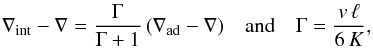 (7)where
Γ is the ratio of the energy transported to the energy lost on the way (i.e. Γ equals the
Peclet number over 6), with v and ℓ the typical velocity
and mean free path of the motions.
(7)where
Γ is the ratio of the energy transported to the energy lost on the way (i.e. Γ equals the
Peclet number over 6), with v and ℓ the typical velocity
and mean free path of the motions.
We now turn to turbulence, which originates mainly from differential rotation, both
vertical (producing vertical shears) and horizontal (producing horizontal shears creating
horizontal turbulence). The (vertical) shear instability is produced by a significant
difference Δv of velocity between nearby layers of the different vertical
coordinates r. In a shear, there is an excess energy by unit of mass and
surface,  (8)locally present in
the differential motions with respect to the case of an average velocity. The Richardson
criterion defines the occurrence of shear instability over the zone considered in
r. If the excess energy in the shear is greater than the work necessary
for overcoming the stable temperature and μ-gradients, we get the usual
Richardson criterion (see also Sect. 4.3).
(8)locally present in
the differential motions with respect to the case of an average velocity. The Richardson
criterion defines the occurrence of shear instability over the zone considered in
r. If the excess energy in the shear is greater than the work necessary
for overcoming the stable temperature and μ-gradients, we get the usual
Richardson criterion (see also Sect. 4.3).
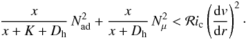
The horizontal turbulence intervenes by changing the μ-gradients. Talon & Zahn (1997) have shown that the
coefficient of horizontal turbulence Dh plays the same role as
the thermal diffusivity in the previous expression (7) and write 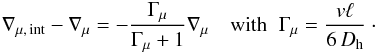 (9)With
proper account of heat losses and horizontal turbulence, the modified Richardson criterion
for shear instability becomes (Talon & Zahn
1997),
(9)With
proper account of heat losses and horizontal turbulence, the modified Richardson criterion
for shear instability becomes (Talon & Zahn
1997), 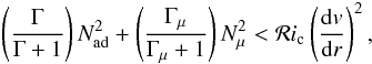 (10)
(10) (11)The
standard value of ℛic = 1/4. Following
Talon & Zahn (1997), we write, with
x = v ℓ/6,
(11)The
standard value of ℛic = 1/4. Following
Talon & Zahn (1997), we write, with
x = v ℓ/6,
 (12)The
heat transport by Dh adds its effects to K.
Assuming that the shear diffusion coefficient
Dshear = (1/3)v ℓ = 2x
(the transport concerns the vertical direction) is small with respect to
K and Dh, Talon & Zahn (1997) have obtained Dshear
taking account of horizontal turbulence and heat losses. This applies to a spherical fluid
element. If not, the result for x has to be multiplied by
(12)The
heat transport by Dh adds its effects to K.
Assuming that the shear diffusion coefficient
Dshear = (1/3)v ℓ = 2x
(the transport concerns the vertical direction) is small with respect to
K and Dh, Talon & Zahn (1997) have obtained Dshear
taking account of horizontal turbulence and heat losses. This applies to a spherical fluid
element. If not, the result for x has to be multiplied by
 as in (3).
2.4. Limit for thermohaline instability
If there is no energy available from the differential rotation for shear instability, the
second member of (12) is zero. Then, if we
also ignore the horizontal turbulence, we just get the limit
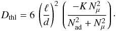 (13)This
is the same as (3), and it shows the
presence of a term depending on the μ-gradient at the denominator. For
thermohaline mixing, ∇μ and
(13)This
is the same as (3), and it shows the
presence of a term depending on the μ-gradient at the denominator. For
thermohaline mixing, ∇μ and  are
negative, thus the diffusion coefficient is evidently positive. As mentioned above,
at the
denominator increases the mixing.
are
negative, thus the diffusion coefficient is evidently positive. As mentioned above,
at the
denominator increases the mixing.
If some horizontal turbulence is present, but no significant shears, we get from (12) 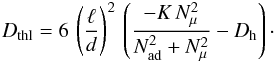 (14)The
first term in the parenthesis is positive and the second negative. Thus, for mixing to
occur, one must have a limit on the value of the horizontal turbulence
Dh,
(14)The
first term in the parenthesis is positive and the second negative. Thus, for mixing to
occur, one must have a limit on the value of the horizontal turbulence
Dh,  (15)A
similar expression, but without the term in the
denominator, has been obtained by Denissenkov &
Pinsonneault (2008). In general, the numerical calculations show that
Dh is smaller than K. However, for
thermohaline mixing to occur, it is necessary that the system is stable at the beginning
(before the slow descending motions), thus
(15)A
similar expression, but without the term in the
denominator, has been obtained by Denissenkov &
Pinsonneault (2008). In general, the numerical calculations show that
Dh is smaller than K. However, for
thermohaline mixing to occur, it is necessary that the system is stable at the beginning
(before the slow descending motions), thus  ,
this means that the right hand side of (15) may be much smaller than K. Thus,
Dh becomes a factor that may cancel the large parenthesis in
(14) and stop the mixing. This is
consistent: when the differences of μ are small with respect to the
stabilizing effect of the T-gradient, turbulence may easily kill the
thermohaline mixing.
,
this means that the right hand side of (15) may be much smaller than K. Thus,
Dh becomes a factor that may cancel the large parenthesis in
(14) and stop the mixing. This is
consistent: when the differences of μ are small with respect to the
stabilizing effect of the T-gradient, turbulence may easily kill the
thermohaline mixing.
As a numerical example, we consider the 1.25 M⊙ model discussed in Sect. 2.2. In this example, the right hand side of (15) is one to two orders of magnitude larger than Dh, implying that the adopted horizontal turbulence does not inhibit the thermohaline mixing. However, the situation may not be so simple. As mentioned, there is a great uncertainty in the size of the horizontal turbulence, so three different expressions have been proposed (Zahn 1992; Maeder 2003; Mathis et al. 2004). Charbonnel & Lagarde (2010) have taken the lowest bound of the first one. The last two, likely more physical (Maeder 2009), give similar numerical values, larger by four to five orders of magnitude than the first one. If applicable, such high values of Dh are sufficient to kill the thermohaline mixing. Thus, the problem of the thermohaline mixing remains open, and we see that a key to its solution lies in better knowledge of the horizontal turbulence in stars, in addition to the proper choice of the geometrical parameters of the fluid elements.
2.5. Semiconvective diffusion
We now turn to semiconvection, where the expression of the diffusion coefficient is
related to that of the thermohaline mixing. Formally, semiconvection occurs when the
thermal gradient ∇ lies midway between the condition of stability predicted by the Ledoux
criterion and the instability predicted by Schwarzschild’s criterion,  (16)where ∇int
is very close to ∇ad in stellar interiors. The velocity of the semiconvective
mixing is also given by (4) as for
thermohaline mixing. The blobs being in dynamical equilibrium, the equation of state
implies
(16)where ∇int
is very close to ∇ad in stellar interiors. The velocity of the semiconvective
mixing is also given by (4) as for
thermohaline mixing. The blobs being in dynamical equilibrium, the equation of state
implies  ,
where ΔT for a blob displaced over a distance Δr is
,
where ΔT for a blob displaced over a distance Δr is
 .
Taking Eqs. (2) and (7) into account, we obtain a coefficient of
semiconvective diffusion (Maeder 2009),
.
Taking Eqs. (2) and (7) into account, we obtain a coefficient of
semiconvective diffusion (Maeder 2009),
 (17)For
Γ tending towards infinity (adiabatic case), one gets the coefficient obtained by Langer et al. (1983). However, semiconvection arises
from nonadiabatic effects, and in stellar interiors, Γ lies between 10-2 and
10-3. Thus, the numerical coefficient
(17)For
Γ tending towards infinity (adiabatic case), one gets the coefficient obtained by Langer et al. (1983). However, semiconvection arises
from nonadiabatic effects, and in stellar interiors, Γ lies between 10-2 and
10-3. Thus, the numerical coefficient  in front of (17) is within this order of
magnitude.
in front of (17) is within this order of
magnitude.
3. Instabilities in rotating stars
3.1. The coupling of the Rayleigh-Taylor and shear instabilities
The effects of shears, thermal diffusion, thermohaline mixing, and horizontal turbulence are all already included in Eq. (12). However, we must also account for the stabilizing or destabilizing effects related to the distribution of the specific angular momentum j = ϖ2 Ω. Indeed, if a (descending) salt finger brings more specific angular momentum inwards than at present in the surrounding medium, this difference of j will tend to bring the fluid element back to its initial position after some oscillations of frequency NΩ, thus the medium is stable. In contrast, if the salt finger brings less specific angular momentum than exists in the surroundings, it tends to continue on its way, and an instability is produced. An analogous discussion can be made for outwards motions. This is well known from the Rayleigh instability criterion: a medium with j decreasing outwards is unstable.
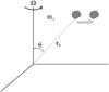 |
Fig. 1 Geometry data concerning the Rayleigh-Taylor instability. |
To examine this effect closely, we consider a star in differential rotation. For now, we
do not need to more specify the dependence of the angular velocity Ω on the spatial
variables. We consider a fluid element at a distance ϖ0 and
move it outwards, as illustrated in Fig. 1, to a very
close point at distance ϖ. The difference in the centrifugal forces
acting on the blob by unit of mass may be written
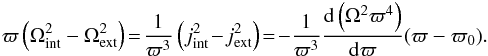 (18)The
work
(18)The
work  delivered by the bubble to the medium during this small displacement is
 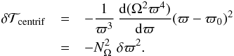 (19)If
Ω decreases very fast with increasing ϖ,
(19)If
Ω decreases very fast with increasing ϖ,
 may be
negative. This means that the motion of the bubble spontaneously delivers some work
to the medium, which is thus unstable. In contrast, the opposite, if
is positive,
one has to give some energy to the bubble in order to move it outwards. The medium is
stable. This leads to the Rayleigh criterion for the stability of a distribution of
angular momentum,
may be
negative. This means that the motion of the bubble spontaneously delivers some work
to the medium, which is thus unstable. In contrast, the opposite, if
is positive,
one has to give some energy to the bubble in order to move it outwards. The medium is
stable. This leads to the Rayleigh criterion for the stability of a distribution of
angular momentum, 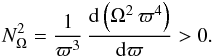 (20)We
emphasize that the above effects of the work made by the centrifugal force leading to
Rayleigh criterion (20) and the effects of
shears as expressed by (8) are two
different physical effects. In some particular hydrodynamic situations, these two effects
can be treated separately. For example, in plane parallel flows with different velocities,
the problem of centrifugal force is not relevant. In contrast, in a differentially
rotating star, both shear effects and angular momentum effects may influence the stability
and should then be treated simultaneously.
(20)We
emphasize that the above effects of the work made by the centrifugal force leading to
Rayleigh criterion (20) and the effects of
shears as expressed by (8) are two
different physical effects. In some particular hydrodynamic situations, these two effects
can be treated separately. For example, in plane parallel flows with different velocities,
the problem of centrifugal force is not relevant. In contrast, in a differentially
rotating star, both shear effects and angular momentum effects may influence the stability
and should then be treated simultaneously.
The displacement of a fluid element implies the exchange of bubbles, leading to some
mixed fluid element with an average spatial velocity. As recalled above, this makes an
energy (1/4) (δv)2 available by unit of
mass. In a star with differential rotation of the “shellular” form Ω(r),
the velocity difference δv is
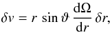 (21)where
ϑ is the colatitude of the point considered (cf. Fig. 1). Thus, an energy
(21)where
ϑ is the colatitude of the point considered (cf. Fig. 1). Thus, an energy
 is made available during an exchange,
  (22)If,
this energy available from the shear is less than the energy (20) necessary to destabilize the angular
momentum distribution, the medium is stable, i.e., if
(22)If,
this energy available from the shear is less than the energy (20) necessary to destabilize the angular
momentum distribution, the medium is stable, i.e., if
 (23)In
the equatorial regions for a case with Ω(r), this can be written as
(23)In
the equatorial regions for a case with Ω(r), this can be written as
 (24)or,
in terms of Ω, as
(24)or,
in terms of Ω, as  (25)The
equality of the two members of this expression gives a quadratic equation in
(dΩ/dr), the solution of which is
(25)The
equality of the two members of this expression gives a quadratic equation in
(dΩ/dr), the solution of which is 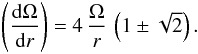 (26)To
be consistent with a solution in the absence of shear, we take the minus sign in the above
expression. This means that to be stable, Ω(r) should not decrease faster
than a limiting Ω-distribution,
(26)To
be consistent with a solution in the absence of shear, we take the minus sign in the above
expression. This means that to be stable, Ω(r) should not decrease faster
than a limiting Ω-distribution, 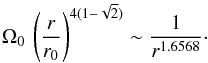 (27)If Ω decreases
outwards faster than this limit, the medium is unstable. Rotation laws of the form
1/rα with
α between 1.6568 and 2.0 are predicted to be stable by the usual
Rayleigh criterion, while if we also account for the excess of energy available in the
shear motions they are unstable. It is clear that there is no reason to ignore the excess
of energy available in shear motions, which contribute to destabilizing the system.
Therefore in a differentially rotating star, the Rayleigh criterion must be modified (see
Sect. 4.1).
(27)If Ω decreases
outwards faster than this limit, the medium is unstable. Rotation laws of the form
1/rα with
α between 1.6568 and 2.0 are predicted to be stable by the usual
Rayleigh criterion, while if we also account for the excess of energy available in the
shear motions they are unstable. It is clear that there is no reason to ignore the excess
of energy available in shear motions, which contribute to destabilizing the system.
Therefore in a differentially rotating star, the Rayleigh criterion must be modified (see
Sect. 4.1).
Reciprocally, when shear instability is considered in a rotating star, the stabilizing or destabilizing effect of the Ω-distribution must also be accounted for. Below, the two effects are coupled and considered simultaneously. This leads to some modifications of well-known criteria.
3.2. A more general coupling
Here we try to be more general and simultaneously consider various effects that may influence the stability of the medium in a rotating star with Ω(r):
-
the effects of thermal gradients;
-
the thermohaline mixing;
-
the semiconvective diffusion;
-
the shear mixing to the local excess of energy in differential rotating layers;
-
the stabilizing or destabilizing effect of the distribution of angular momentum;
-
the radiative losses;
-
the transport of heat by the horizontal turbulence;
-
the element diffusion in the medium due to the horizontal turbulence.
Following Eq. (10) and the previous
section, and taking into account that centrigugal force operates orthogonally to the
rotation axis, we write, for the complete form of the instability expression,
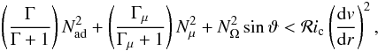 (28)where
the standard value of ℛic is 1/4 and we
have accounted for the effect of the distribution of the specific angular momentum
j on the stability. Making the same transformation
x = v ℓ/6 as in
(12), we get the following instability
condition,
(28)where
the standard value of ℛic is 1/4 and we
have accounted for the effect of the distribution of the specific angular momentum
j on the stability. Making the same transformation
x = v ℓ/6 as in
(12), we get the following instability
condition, 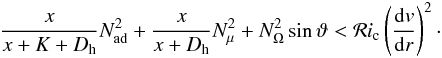 (29)This
general equation may be used to get the total resulting diffusion coefficient
Dtot = 2x of the chemical elements in a
star, considering the many effects involved. The stability condition may be written as a
quadratic equation of the form
Ax2 + Bx + C > 0,
(29)This
general equation may be used to get the total resulting diffusion coefficient
Dtot = 2x of the chemical elements in a
star, considering the many effects involved. The stability condition may be written as a
quadratic equation of the form
Ax2 + Bx + C > 0,
![Mathematical equation: \begin{eqnarray} &&\left[N^2_{\mathrm{ad}}+N^2_{\mu}+N^2_{{\Omega}-\delta v} \right]\, x^2\nonumber \\ &&\qquad + \left[N^2_{\mathrm{ad}}D_{\mathrm{h}}+N^2_{\mu}(K+D_{\mathrm{h}})+ N^2_{{\Omega} -\delta v} (K+2 D_{\mathrm{h}}) \right] \, x\nonumber \\ &&\qquad + N^2_{{\Omega}-\delta v} (D_{\mathrm{h}}K+ D^2_{\mathrm{h}}) > 0 , \label{2ndeq} \end{eqnarray}](/articles/aa/full_html/2013/05/aa20936-12/aa20936-12-eq117.png) (30)with
(30)with
 (31)Expression of
 is a modified
form of the Rayleigh oscillation frequency, accounting for both the angular momentum
distribution and the excess of energy in the shear. Equation (30) is the general equation, which should
generally be considered in a rotating star to account for the various effects mentioned
above. It contains the Schwarzschild, the Ledoux, the Solberg-Høiland, the
Rayleigh-Taylor, the Richardson, and the GSF criteria with radiative losses and horizontal
turbulence all in one single expression. Simplifications are possible, but they should be
justified.
is a modified
form of the Rayleigh oscillation frequency, accounting for both the angular momentum
distribution and the excess of energy in the shear. Equation (30) is the general equation, which should
generally be considered in a rotating star to account for the various effects mentioned
above. It contains the Schwarzschild, the Ledoux, the Solberg-Høiland, the
Rayleigh-Taylor, the Richardson, and the GSF criteria with radiative losses and horizontal
turbulence all in one single expression. Simplifications are possible, but they should be
justified.
In the first evolutionary phases, is generally
likely to have a stabilizing influence since the Ω-gradient is not very steep. This means
that the instabilities could be somehow reduced in the equatorial regions. In the advanced
phases after the end of the He-burning phases, may be
destabilizing over very limited regions (Hirschi &
Maeder 2010), where equatorial instabilities may be favored.
At the equator, coordinates ϖ and r coincide, the
effect of the centrifugal force is maximum, while at the pole this effect disappears, and
vanishes. The
distribution of the instability inside the star is no longer spherically symmetric.
Indeed, all properties of rotating stars are two-dimensional: the shape, the isobars, the
meridional circulation, and the various instabilities have a dependence on colatitude
ϑ. The usual practice (Kippenhahn
& Thomas 1970) is to consider the equations of structure at an average
radius rP, such that the volume of the sphere
of radius rP is equal to the real volume of
the oblate rotating star. This is also valid for differentially rotating star with
shellular rotation (Meynet & Maeder 1997).
The radius rP is equivalent to the radius of
the oblate star at colatitude ϑ given by
P2(cosϑ) = 0, i.e.
cos2ϑ = 1/3, which corresponds to
ϑ = 54.7 degrees. Thus, in Eq. (31), we put  and we may thus keep the
advantages of the 1D modeling. However, all these procedures may satisfactorily apply for
the lower rotation velocities, while for high velocities, there may be significant
differences from the complex 2D reality of rotating stars.
and we may thus keep the
advantages of the 1D modeling. However, all these procedures may satisfactorily apply for
the lower rotation velocities, while for high velocities, there may be significant
differences from the complex 2D reality of rotating stars.
3.3. The general solution
In stellar models, it is often considered that the total diffusion coefficient
Dtot is the sum of several diffusion coefficients
Di, each one corresponding to an instability
i,  (32)Such a summation of
coefficients Di is undoubtedly wrong! The
solution to an equation of the second degree like (30) is not the sum of the limits in some particular cases. The
solution is that of the complete equation. This leads to introducing correlations between
the various effects in the form of products of terms appearing in the coefficients
A, B and C of the quadratic Eq.
(30). These are
(32)Such a summation of
coefficients Di is undoubtedly wrong! The
solution to an equation of the second degree like (30) is not the sum of the limits in some particular cases. The
solution is that of the complete equation. This leads to introducing correlations between
the various effects in the form of products of terms appearing in the coefficients
A, B and C of the quadratic Eq.
(30). These are ![Mathematical equation: \begin{eqnarray} &&A= \left[N^2_{\mathrm{ad}}+N^2_{\mu}+N^2_{{\Omega}-\delta v} \right] ,\\ \nonumber && B= N^2_{\mathrm{ad}}D_{\mathrm{h}}+N^2_{\mu}(K+D_{\mathrm{h}})+ N^2_{{\mathrm{\Omega}} -\delta v} (K+2 D_{\mathrm{h}}) ,\\ \nonumber &&C=N^2_{{\Omega}-\delta v} (D_{\mathrm{h}}K+ D^2_{\mathrm{h}}) . \label{BC} \end{eqnarray}](/articles/aa/full_html/2013/05/aa20936-12/aa20936-12-eq133.png) (33)The
solution of (30) brings coupling of all
intervening factors. We notice in particular the cross-products of the heat losses and of
the horizontal turbulence with the effects of the thermal, μ-, and
Ω-gradients. There are also products of these three gradients and direct products of heat
losses and horizontal turbulence. This indicates that the full solution of the diffusion
coefficient D = |2x| depends on the coupling of the
various physical effects being considered and is by no means a sum like (32).
(33)The
solution of (30) brings coupling of all
intervening factors. We notice in particular the cross-products of the heat losses and of
the horizontal turbulence with the effects of the thermal, μ-, and
Ω-gradients. There are also products of these three gradients and direct products of heat
losses and horizontal turbulence. This indicates that the full solution of the diffusion
coefficient D = |2x| depends on the coupling of the
various physical effects being considered and is by no means a sum like (32).
4. Some stability criteria reconsidered
The above results lead us to reconsider some basic stability criteria in differentially
rotating stars, which indeed only account for one specific aspect of the instability and
ignore other ones, which are unavoidably present in rotating stars. In particular, we see
that the complete Eq. (30) contains the term
. In agreement
with the result of (3.1), the term
should always be
considered instead of  in the relevant
criteria.
in the relevant
criteria.
4.1. A modified Rayleigh-Taylor criterion
The usual Rayleigh-Taylor criterion for the stability of a rotating flow (in absence of
gravity) is ![Mathematical equation: \begin{equation} N^2_{\Omega} > 0 , \\ [2mm] \mathrm{with} \quad N^2_{\Omega} = \frac{1}{\varpi^3} \, \frac{{\rm d}\left( \Omega^2 \, \varpi^4 \right) }{{\rm d}\varpi} \cdot \label{classicRT} \end{equation}](/articles/aa/full_html/2013/05/aa20936-12/aa20936-12-eq136.png) (34)It expresses that
for a rotating medium to be stable, the angular momentum must increase with the distance
to the rotation axis.
(34)It expresses that
for a rotating medium to be stable, the angular momentum must increase with the distance
to the rotation axis.
If in the general Eq. (30) we put
K and Dh equal to zero and if we also do
not consider the effects of thermal and μ-gradients, we are left with the
stability condition  (35)At a colatitude
ϑ in a star, we should consider this new form of the criterion for the
stability of differential rotation, If positive, it means that the excess energy in the
differential rotation is unable to destabilize a stable distribution of angular momentum.
If negative, the medium is unstable.
(35)At a colatitude
ϑ in a star, we should consider this new form of the criterion for the
stability of differential rotation, If positive, it means that the excess energy in the
differential rotation is unable to destabilize a stable distribution of angular momentum.
If negative, the medium is unstable.
Indeed, the Rayleigh-Taylor criterion (34) may predict the stability of a given differential rotation law, while in fact it would be unstable according to (35), as discussed in Sect. 3.1. The usual Rayleigh-Taylor criterion (34) should never apply as such to a rotating star, since the shears also favor instability.
4.2. A modified form of the Solberg-Høiland criterion
We first recall the usual Solberg-Høiland criterion for convective stability,
 (36)This to some extent
combines the Ledoux and the Rayleigh-Taylor criteria. It expresses the stability with
respect to convective motions (at the dynamical timescale
R3/(GM)), which also
accounts for the stability of the rotation law.
(36)This to some extent
combines the Ledoux and the Rayleigh-Taylor criteria. It expresses the stability with
respect to convective motions (at the dynamical timescale
R3/(GM)), which also
accounts for the stability of the rotation law.
If in the general Eq. (30) we put
K and Dh equal to zero, the terms
B and C in (34) are zero so we are left with the condition  (37)or more explicitely
 (38)This
is the modified form of the Solberg-Høiland criterion for stability, accounting for the
fact that both the distribution of j and the energy excess in
differential rotation are considered simultaneously. The last term on the left-hand side
may reduce stability. Thus in a differentially rotating star, a situation considered as
stable according to (36) could in reality
be unstable.
(38)This
is the modified form of the Solberg-Høiland criterion for stability, accounting for the
fact that both the distribution of j and the energy excess in
differential rotation are considered simultaneously. The last term on the left-hand side
may reduce stability. Thus in a differentially rotating star, a situation considered as
stable according to (36) could in reality
be unstable.
The Solberg-Høiland criterion does not account for radiative losses, which would introduce the term Γ/(Γ + 1) in front of the first term in Eqs. (36) and (38). This would lead to a dependence on the thermal timescale. It does not account for viscosity due to turbulence, which would introduce a dependence on the viscous timescale. The Solberg-Høiland instability essentially obeys the dynamical timescale. The terms accounting for radiative losses and (turbulent) viscosity will appear below in the so-called GSF criterion. In such a case, one would have a kind of semiconvective diffusion like (17), including in addition the effects of rotation. The characteristic timescales is determined by the thermal timescale rather than by the dynamical timescale.
4.3. The Richardson criterion
The usual expression of the Richardson criterion for shear instability in a star with
shellular rotation is  (39)It
expresses that if the excess energy in the shear overcomes the restoring energy available
in the stable temperature- and μ-gradients, then mixing occurs.
(39)It
expresses that if the excess energy in the shear overcomes the restoring energy available
in the stable temperature- and μ-gradients, then mixing occurs.
If we ignore thermal losses and horizontal turbulence, the modified form of the Richardson criterion is identical to the above modified expression (38) of the Solberg-Høiland criterion, since the shear effects have to be considered together with those regarding the stability of the angular momentum distribution.
If the thermal losses with the term K are considered and not the
horizontal turbulence, the stability relation (30) becomes ![Mathematical equation: \begin{eqnarray} \left[N^2_{\mathrm{ad}}+N^2_{\mu}+N^2_{{\Omega}-\delta v} \right]\, x + \left[N^2_{\mu}\, K+ N^2_{{\mathrm{\Omega}} -\delta v} \, K \right] > 0 . \label{2ndeqK} \end{eqnarray}](/articles/aa/full_html/2013/05/aa20936-12/aa20936-12-eq144.png) (40)The
corresponding diffusion coefficient
Dshear = 2x is
(40)The
corresponding diffusion coefficient
Dshear = 2x is  (41)This
is the diffusion coefficient for the effects of shear, accounting for the
T- and μ-gradients, for the thermal losses, and for
the Rayleigh-Taylor instability. The complete form of the stability criterion, including
thermal losses and horizontal turbulence, is given by Eq. (30).
(41)This
is the diffusion coefficient for the effects of shear, accounting for the
T- and μ-gradients, for the thermal losses, and for
the Rayleigh-Taylor instability. The complete form of the stability criterion, including
thermal losses and horizontal turbulence, is given by Eq. (30).
4.4. The GSF criterion
The Goldreich-Schubert-Fricke (GSF) criterion (Goldreich
& Schubert 1967; Fricke 1968)
considers the instability of a stellar rotation law subject to thermal diffusivity
K and to viscosity ν. Instability occurs for each of
the two conditions, ![Mathematical equation: \begin{eqnarray} \label{GSF1} && \frac{\nu}{K} \; N^2_{\mathrm{T, ad}}+N^2_{\Omega} < 0 \\[2mm] \label{GSF2} &&\mathrm{and} \quad \left|\varpi \frac{\partial \Omega^2} {\partial z} \right| > \frac{\nu}{K} \; N^2_{\mathrm{T, ad}} . \end{eqnarray}](/articles/aa/full_html/2013/05/aa20936-12/aa20936-12-eq148.png) The
first inequality expresses the same idea as the Solberg-Høiland criterion, including
thermal diffusivity. The second relation expresses the instability related to the
differential rotation in the direction parallel to the rotation axis.
The
first inequality expresses the same idea as the Solberg-Høiland criterion, including
thermal diffusivity. The second relation expresses the instability related to the
differential rotation in the direction parallel to the rotation axis.
The ratio ν/K can also be expressed
in terms of Γ as in Sect. 2.3, where we see a term
Γ/(Γ + 1) in front of  . The
viscosity is
ν = (1/3) v ℓ
and Γ = v ℓ/(6K).
Formally, there is a correspondence
Γ = ν/(2K). The difference between
a term such as in Eq. (42) and terms like
Γ/(Γ + 1) comes from two facts:
. The
viscosity is
ν = (1/3) v ℓ
and Γ = v ℓ/(6K).
Formally, there is a correspondence
Γ = ν/(2K). The difference between
a term such as in Eq. (42) and terms like
Γ/(Γ + 1) comes from two facts:
-
1.
In expressing Γ, account is given to the geometrical shape of the fluid element supposed to experience radiative losses, while in Eq. (42) this is not done.
-
2.
Also, as shown by Maeder (1995, 2009), in the general case of radiative losses one must consider the ratio Γ/(Γ + 1) in front of
. It is
only for an extreme conductivity (Γ → 0) of the medium that one may just write Γ or
ν/K. In contrast, Γ → ∞ and
the term in front of is 1 in
the perfect adiabatic case.
From these two remarks, one sees that the following writing of the standard GSF criterion
is more appropriate, ![Mathematical equation: \begin{eqnarray} \label{GSF11} && \left( \frac{\Gamma}{\Gamma+1}\right) \, N^2_{\mathrm{T, ad}}+N^2_{\Omega} \, \sin \vartheta < 0 \\ [2mm] \label{GSF22} && \mathrm{and} \quad \left|\varpi \frac{\partial \Omega^2} {\partial z} \right| > \left( \frac{\Gamma}{\Gamma+1}\right) \, N^2_{\mathrm{T, ad}} , \end{eqnarray}](/articles/aa/full_html/2013/05/aa20936-12/aa20936-12-eq157.png) with
the same notations as in Sect. 2.3.
with
the same notations as in Sect. 2.3.
The effect of μ-gradient can also be accounted for, as can the
diffusivity of chemical elements, due in particular to the horizontal turbulence. The
instability is then triple diffusive. In a rotating star, the horizontal turbulence is a
major diffusive process, and its effects on the GSF instability have been studied (Hirschi & Maeder 2010). As for previous
criteria, we also need here to account for the excess energy present in the shears. We do
it in the same way as before by replacing by
. The first
expression of the GSF instability criterion is thus  (46)The
second is
(46)The
second is  (47)These
conditions are easier to realize than the standard ones, which means that the domain of
the GSF instability is somehow extended by the inclusion of the excess energy in the
shear. As shown previously (Hirschi & Maeder
2010), the GSF instability can be very large locally in presupernova stages, but
the zones over which the GSF instability is acting are very narrow. It may be interesting
to examine whether the above expressions
(47)These
conditions are easier to realize than the standard ones, which means that the domain of
the GSF instability is somehow extended by the inclusion of the excess energy in the
shear. As shown previously (Hirschi & Maeder
2010), the GSF instability can be very large locally in presupernova stages, but
the zones over which the GSF instability is acting are very narrow. It may be interesting
to examine whether the above expressions
are changing the results. As a matter of fact, we see that the first criterion is equivalent to our general stability Eq. (30). The solution is given by the root of this quadratic equation.
5. Conclusions
We have simultaneously considered various instabilities in differentially rotating stars and given a general equation expressing the instability conditions with respect to an ensemble of effects, including horizontal turbulence. This introduces some coupling between the instabilities. We suggested that in rotating stars some instabilities should never be dissociated. In particular the instability of rotation law expressed by Rayleigh criterion and the shear instability should always be considered simultaneously. Modeling the instabilities in 1D models of stars with low or moderate rotation velocities is possible by considering the effects at the root of P2(cosϑ) = 0. In future work now in preparation, we will examine the consequences of the present approach on the mixing in stellar interiors.
Acknowledgments
G.M., N.L., and C.C. acknowledge different sources of support from the Swiss National Fund.
References
- Brown, J., Garaud, P., & Stellmach, S. 2012 [arXiv:1212.1688] [Google Scholar]
- Cantiello, M., & Langer, N. 2010, A&A, 521, A9 [NASA ADS] [CrossRef] [EDP Sciences] [Google Scholar]
- Chaboyer, B., & Zahn, J.-P. 1992, A&A, 253, 173 [NASA ADS] [Google Scholar]
- Chandrasekhar, S. 1961, Hydrodynamic and hydromagnetic stability (New York: Dover Publications) [Google Scholar]
- Charbonnel, C., & Lagarde, N. 2010, A&A, 522, A10 [NASA ADS] [CrossRef] [EDP Sciences] [MathSciNet] [PubMed] [Google Scholar]
- Charbonnel, C., & Zahn, J.-P. 2007, A&A, 467, L15 [NASA ADS] [CrossRef] [EDP Sciences] [Google Scholar]
- Denissenkov, P. A. 2010, ApJ, 723, 563 [NASA ADS] [CrossRef] [Google Scholar]
- Denissenkov, P. A., & Merryfield, W. J. 2011, ApJ, 727, L8 [NASA ADS] [CrossRef] [Google Scholar]
- Denissenkov, P. A., & Pinsonneault, M. 2008, ApJ, 684, 626 [NASA ADS] [CrossRef] [Google Scholar]
- Endal, A. S., & Sofia, S. 1978, ApJ, 220, 279 [NASA ADS] [CrossRef] [Google Scholar]
- Fricke, K. 1968, ZAp, 68, 317 [Google Scholar]
- Goldreich, P., & Schubert, G. 1967, ApJ, 150, 571 [NASA ADS] [CrossRef] [Google Scholar]
- Hirschi, R., & Maeder, A. 2010, A&A, 519, A16 [NASA ADS] [CrossRef] [EDP Sciences] [Google Scholar]
- Kippenhahn, R., & Thomas, H.-C. 1970, in IAU Colloq. 4: Stellar Rotation, ed. A. Slettebak, 20 [Google Scholar]
- Kippenhahn, R., Ruschenplatt, G., & Thomas, H.-C. 1980, A&A, 91, 175 [NASA ADS] [Google Scholar]
- Lagarde, N., Romano, D., Charbonnel, C., et al. 2012, A&A, 542, A62 [NASA ADS] [CrossRef] [EDP Sciences] [Google Scholar]
- Langer, N., Fricke, K. J., & Sugimoto, D. 1983, A&A, 126, 207 [NASA ADS] [Google Scholar]
- Maeder, A. 1995, A&A, 299, 84 [NASA ADS] [Google Scholar]
- Maeder, A. 2003, A&A, 399, 263 [NASA ADS] [CrossRef] [EDP Sciences] [Google Scholar]
- Maeder, A. 2009, Physics, Formation and Evolution of Rotating Stars (Berlin, Heidelberg: Springer) [Google Scholar]
- Mathis, S., Palacios, A., & Zahn, J.-P. 2004, A&A, 425, 243 [NASA ADS] [CrossRef] [EDP Sciences] [Google Scholar]
- Meynet, G., & Maeder, A. 1997, A&A, 321, 465 [NASA ADS] [Google Scholar]
- Talon, S., & Zahn, J.-P. 1997, A&A, 317, 749 [Google Scholar]
- Théado, S., & Vauclair, S. 2012, ApJ, 744, 123 [NASA ADS] [CrossRef] [Google Scholar]
- Traxler, A., Garaud, P., & Stellmach, S. 2011, ApJ, 728, L29 [NASA ADS] [CrossRef] [Google Scholar]
- Ulrich, R. K. 1972, ApJ, 172, 165 [NASA ADS] [CrossRef] [Google Scholar]
- Vauclair, S., & Théado, S. 2012, ApJ, 753, 49 [NASA ADS] [CrossRef] [Google Scholar]
- Wachlin, F. C., Miller Bertolami, M. M., & Althaus, L. G. 2011, A&A, 533, A139 [NASA ADS] [CrossRef] [EDP Sciences] [Google Scholar]
- Wasiutynski, J. 1946, Astrophys. Norvegica, 4, 1 [NASA ADS] [Google Scholar]
- Zahn, J.-P. 1992, A&A, 265, 115 [NASA ADS] [Google Scholar]
All Figures
|
Fig. 1 Geometry data concerning the Rayleigh-Taylor instability. |
| In the text | |
Current usage metrics show cumulative count of Article Views (full-text article views including HTML views, PDF and ePub downloads, according to the available data) and Abstracts Views on Vision4Press platform.
Data correspond to usage on the plateform after 2015. The current usage metrics is available 48-96 hours after online publication and is updated daily on week days.
Initial download of the metrics may take a while.