| Issue |
A&A
Volume 550, February 2013
|
|
|---|---|---|
| Article Number | A73 | |
| Number of page(s) | 17 | |
| Section | Astronomical instrumentation | |
| DOI | https://doi.org/10.1051/0004-6361/201219781 | |
| Published online | 29 January 2013 | |
Sparse component separation for accurate cosmic microwave background estimation
Laboratoire AIM, UMR CEA-CNRS-Paris 7, Irfu, SAp/SEDI, Service d’Astrophysique, CEA Saclay, 91191 Gif-sur-Yvette Cedex, France
e-mail: jbobin@cea.fr
Received: 8 June 2012
Accepted: 28 September 2012
The cosmic microwave background (CMB) is of premier importance for cosmologists in studying the birth of our universe. Unfortunately, most CMB experiments, such as COBE, WMAP, or Planck do not directly measure the cosmological signal, because the CMB is mixed up with galactic foregrounds and point sources. For the sake of scientific exploitation, measuring the CMB requires extracting several different astrophysical components (CMB, Sunyaev-Zel’dovich clusters, galactic dust) from multiwavelength observations. Mathematically speaking, the problem of disentangling the CMB map from the galactic foregrounds amounts to a component or source separation problem. In the field of CMB studies, a wide range of source separation methods have been applied that all differ in the way they model the data and in the criteria they rely on to separate components. Two main difficulties are i) that the instrument’s beam varies across frequencies and ii) that the emission laws of most astrophysical components vary across pixels. This paper aims at introducing a very accurate modeling of CMB data, based on sparsity to account for beams’ variability across frequencies, as well as for spatial variations of the components’ spectral characteristics. Based on this new sparse modeling of the data, a sparsity-based component separation method coined local-generalized morphological component analysis (L-GMCA) is described. Extensive numerical experiments have been carried out with simulated Planck data. These experiments show the high efficiency of the proposed component separation methods for estimating a clean CMB map with a very low foreground contamination, which makes L-GMCA of prime interest for CMB studies.
Key words: cosmic background radiation / methods: data analysis / methods: statistical
© ESO, 2013
1. Introduction
A very large number of experiments have been dedicated to studying the cosmic microwave background (CMB) anisotropies. Launched in 2001, the WMAP satellite has been observing the sky in five frequency bands ranging from 22 GHz to 94 GHz (Bennett et al. 2003a). This survey has been providing full-sky maps of the CMB fluctuations up to a resolution of 13.2 arcmin at 94 GHz. More recently, the Planck mission (Planck Collaboration 2006), launched in May 2009, is currently providing full sky observations in 9 frequency bands from 30 GHz to 857 GHz at resolutions ranging from 33 arcmin at 30 GHz to 5 arcmin at 857 GHz. Expected to be released in early 2013, Planck will provide full-sky maps of the CMB anisotropies at an unprecedented resolution of 5 arcmin.
The CMB is generally not observable directly; most CMB experiments such as WMAP or Planck provide multi-wavelength observations in which the CMB is mixed with other astrophysical components. Recovering useful cosmological information requires disentangling the contribution in the CMB data of several astrophysical components, namely CMB itself as well as various foreground components see (Bouchet & Gispert 1999).
The main foreground contributors include:
-
Synchrotron: this emission arises from the acceleration ofcosmic-ray electrons in magnetic fields. It follows a power lawwith a spectral index that varies across pixels from −3.4 and −2,3 (Bennettet al. 2003b). In the Planck data,this component mainly appears at lower frequency observations(typ.ν < 70 GHz).
-
Free-free: the free-free emission develops from the electron-ion scattering. This component has power-law emission with a rather constant spectral index across the sky (around –2.15; Dickinson et al. 2003).
-
Dust emission: this component arises from the thermal radiation of the dust grains of the Milky Way. This emission follows a gray body law that depends on two parameters: dust temperature and spectral index (Finkbeiner et al. 1999). Recent studies involving the joint analysis of IRAS and the 545 GHz and 857 Ghz observations from Planck show significant variations in the dust temperature and spectral index across pixels on both large and small scales (Planck Collaboration 2011a).
-
AME: the AME (anomalous microwave emission) or spinning dust may develop from the emission of spinning dust grains on nanoscale. This component spatially correlates with the thermal dust emission but has an emissivity that roughly follows a power law in the range of frequencies observed by Planck and WMAP (Planck Collaboration 2011c).
-
SZ: the Sunyaev-Zel’Dovich effect results from the interactions of high energy electrons and the CMB through inverse Compton scattering (Sunyaev & Zeldovich 1970). The electromagnetic spectrum of the SZ component is well known and constant across pixels.
-
Point sources: these components are made of two categories, radio and infrared point sources that can be of galactic or extra-galactic origins. Most of the brightest compact sources are found in the ERCSC catalogue provided by the Planck mission (Planck Collaboration 2011b). These point sources have individual electromagnetic spectra.
Unseen by WMAP, the emission of carbon monoxide (CO) will also be seen by Planck in its 100, 217 and 353 GHz channels. The recovery of all these sources falls in the framework of component separation. For an efficient component separation over a large portion of the sky, a range of channels needs to be observed to disambiguate the various foregrounds. Component separation consists of estimating a set of parameters (i.e. mixing matrix, power spectral and spectral index to only name a few) that describes the components of interest, as well as how they contribute to the data. For example, it could be parameters describing the statistical properties such as power spectra, electromagnetic spectra to name only two.
A wide range of component separation techniques have been proposed. They mainly differ from each other in the way they model the data and the assumptions made on the components to be separated. An overview of the major component separation techniques is given in Sect. 2. The modeling of the data is challenging because it involves a wide variety of instrumental and physical phenomena, such as:
-
Instrumental noise: it is generally correlated and nonstationary,because each position in the sky is not observed the same numberof times. The noise variance varies across pixels.
-
Point sources: point sources are very hard to account for in component separation, because each point source has its own electromagnetic spectrum. Therefore the contribution of point sources cannot be defined as a simple spatial template that scales across frequencies.
-
Emissivity variations: it is well established that the emissivity of most foregrounds, such as dust (Planck Collaboration 2011a) or synchrotron (Bennett et al. 2003b), varies across the sky. Again, assuming that the electromagnetic spectrum of these components is constant across pixels is inaccurate.
-
Heterogeneous beams: the observed maps generally have different resolutions; furthermore, the beams are not necessarily isotropic and spatially invariant.
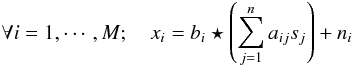
![\begin{eqnarray} x_i [k] = b_i \star \left( \sum_{j=1}^{N_{\rm s}} a_{i, j}[k] s_j[k] \right)+ n_{i}[k]. \label{eq_mixte} \end{eqnarray}](/articles/aa/full_html/2013/02/aa19781-12/aa19781-12-eq19.png) (1)In this equation i is the channel number, k the pixel position, Ns the number of sky emissions, bi the instrument beam (i.e. point spread function), ai,j [k] models for the contribution of source j in channel i, sj is the jth sky component and ni [k] the noise. The observation xi centered on frequency νi is defined as the integration across the detector spectral transmission Ti(μ). In Eq. (1), this integration is hidden in the terms ai,j [k] which can be precisely defined as
(1)In this equation i is the channel number, k the pixel position, Ns the number of sky emissions, bi the instrument beam (i.e. point spread function), ai,j [k] models for the contribution of source j in channel i, sj is the jth sky component and ni [k] the noise. The observation xi centered on frequency νi is defined as the integration across the detector spectral transmission Ti(μ). In Eq. (1), this integration is hidden in the terms ai,j [k] which can be precisely defined as ![\begin{equation*} a_{i,j}[k] = \int_\nu T_{i}(\nu) f_{\nu,j}[k] {\rm d}\nu \end{equation*}](/articles/aa/full_html/2013/02/aa19781-12/aa19781-12-eq29.png) where fν,j [k] stands for the spectral energy distribution (SED) of the component sj at pixel k. If we omit the effect of the beams and assume that the sky component spectral behavior does not vary across the sky (i.e. ai,j [k] is constant for any fixed (i,j)), then the above equation can be recast as
where fν,j [k] stands for the spectral energy distribution (SED) of the component sj at pixel k. If we omit the effect of the beams and assume that the sky component spectral behavior does not vary across the sky (i.e. ai,j [k] is constant for any fixed (i,j)), then the above equation can be recast as  (2)The matrix X represent the observed multichannel data, S the unknown sources, and A the unknown or partially unknown mixing matrix (ai,j the contribution of component sj to the channel i at frequency νi). Therefore, one needs to find S and A from the observed data X alone. This is obviously a very ill-posed problem known, in the statistics community, as blind source separation (BSS; Comon & Jutten 2010). During the last decades, various methods have been introduced to tackle BSS problems. The main differences between all these component separation methods are the statistical assumptions made to differentiate between the sources. A famous example is independent component analysis (Hyvarinen et al. 2001) which relies on the statistical independence of the sources. Although independence is a strong assumption, it is physically acceptable in many cases, and provides much better solutions than using a simple second order decorelation assumption generally obtained with methods such as using principal component analysis (PCA; Hastie et al. 2009). In the field of astrophysics, a very wide range of CMB map estimation techniques have been proposed in the last decades.
In this paper, we first review in Sect. 2 the major classes of component separation methods, and we discuss the advantages and drawbacks of each of them. In Bobin et al. (2007, 2008), we introduced a novel component separation method coined generalized morphological component analysis method (GMCA) which profits from how foreground emissions can be sparsely represented in a well chosen signal representation (e.g. wavelets). The estimation of the components and the unknown coefficients in the mixing matrix is performed by enforcing the sparsity of the components in the wavelet domain. Section 3 discusses the use of sparsity prior for CMB estimation in more details. We show in Sect. 5 how the GMCA method can be modified to properly take into account the different resolutions of the different channels, and the spatial variation of the mixing matrix. Based on this sophisticated data modeling, a novel sparse component separation method local GMCA (L-GMCA) coined is described. Finally, results of extensive numerical experiments are presented in Sect. 6, which shows the advantage on the sparse recovery method over the ILC-based approach. Except for GMCA1, codes relative to these different methods are not public. This makes the comparison between them relatively difficult. However, a first comparison of these methods has been done in (Leach 2008) on full-sky simulated Planck data. Regardless of the kind of approach one adopts, efficient CMB estimation requires an accurate modeling of the data, as well as a robust and effective separation technique. Also, with the future Planck release in 2013, we need to have a much better understanding of what methods work better to recover a high-quality CMB map from full-sky surveys.
2. Overview of CMB recovery methods
One of the first attempts to recover full-sky estimates of the CMB map was made through multichannel Wiener filtering (Bouchet et al. 1999). Since, a very large number of component separation techniques have been proposed to estimate components from CMB data. These methods can be split up into three categories: i) template fitting; ii) statistical methods derived from blind source separation (BSS) and iii) parametric methods. In a nutshell, template fitting techniques (Dunkley et al. 2009) profit from some prior knowledge of spatial templates for the major components to be extracted. Given a parametric modeling of the components, parametric methods (Stolyarov et al. 2005; Eriksen et al. 2008) generally estimate the components’ parameters from their posterior distributions. Finally, inspired by BSS in the statistics community (Comon & Jutten 2010), blind source separation (BSS) techniques (Delabrouille et al. 2009; Bobin et al. 2008a; Bedini et al. 2005) rely on some statistical measure of diversity (i.e. statistical independence or sparsity to name only two) between the sources to separate out the different components. All these component separation methods therefore differ from each other in the way they model the data as well as in the criteria they use to distinguish the sources. In this section we present an overview of the various methods proposed for CMB recovery and discuss their relative advantages and drawbacks.
Template fitting
Having the foregrounds as additional components of the microwave sky, one can perform a fit of the template to the data for foreground analysis. For Nt template vectors, { ti } i = 1,··· ,NT, the template-corrected data has the form at frequency νi (3)where the best-fit amplitude, βj, for each foreground template can be obtained by minimizing
  , where C is the total covariance matrix for the template-corrected data
  . Template-fitting can be performed either in the pixel domain or in harmonic space. Pixel-based implementation allows for incomplete sky coverage, as well as a refined modeling of nonstationary noise at the expense of a more complex modeling of the data: the CMB covariance matrix is large and dense. Conversely, spherical harmonics make the modeling of CMB much simpler but requires crude stationary assumptions for noise. CMB cleaning by template fitting has a number of advantages, starting with its simplicity. The technique makes full use of the spatial information in the template map, which is important for the nonstationary, highly non-Gaussian emission distribution, typical of Galactic foregrounds. There are also disadvantages to this technique because the noise of the template is added to the solution, and imperfect models of the templates could add systematics and non-Gaussianities to the data. We refer the reader to (Dunkley et al. 2009) for a more detailed description of template fitting techniques. Template cleaning of the COBE/FIRAS data reduced a complicated foreground by a factor of ten by using only three spatial templates (Fixsen et al. 1998).
Second order statistical methods
ILC: internal linear combination
In the field of cosmology internal linear combination has ben widely used, (see Eriksen et al. 2004; Hurier et al. 2010; Remazeilles et al. 2011; Delabrouille et al. 2009). In this framework, very little is assumed about the different components to be separated out. The main component is assumed to be the same in all the frequency bands, and the observations are calibrated with respect to this component. Each observation xi is modeled at pixel k as ![\begin{equation} x_{i}[k]=s[k]+f_{i}[k]+n_{i}[k] \end{equation}](/articles/aa/full_html/2013/02/aa19781-12/aa19781-12-eq47.png) (4)where i denotes the frequency channels at frequency νi, fi [k] , and ni [k] are the foregrounds and noise contributions at pixel k, respectively. One then looks for the solution
(4)where i denotes the frequency channels at frequency νi, fi [k] , and ni [k] are the foregrounds and noise contributions at pixel k, respectively. One then looks for the solution ![\begin{equation} \hat{s}[k]=\sum_{i}w_{i}[k]x_{i}[k]. \end{equation}](/articles/aa/full_html/2013/02/aa19781-12/aa19781-12-eq49.png) (5)The simplest version of ILC assumes the weights wi [k] are constant across the sky and therefore are not functions of k. The ILC estimate of the CMB is then obtained by estimating the weights w, which minimize the variance of the estimated CMB map:
(5)The simplest version of ILC assumes the weights wi [k] are constant across the sky and therefore are not functions of k. The ILC estimate of the CMB is then obtained by estimating the weights w, which minimize the variance of the estimated CMB map:  (6)where a is the electromagnetic spectrum of CMB (a vector made of ones for data in thermodynamic units) and ΣX = XXT. Solving the minimization problem in Eq. (6) leads to
  The final CMB map is then
  .
.
Additionally, the ILC solution can be interpreted equivalently as a maximum likelihood estimate assuming that the covariance matrix of the error is the covariance matrix of the data themselves (this assumption is a good approximation when the foregrounds and/or intrumental noise are preeminent). This is equivalent to minimizing the weighted least square of the residual X − as: ŝ = mins(X − as)TΣX-1(X − as). This interpretation makes ILC closely linked to the “best linear unbiased estimator” (a.k.a. BLUE; Kay 1993) in statistics with the assumption that the covariance of the error is identical to the covariance of the data. To improve on this, the map is generally decomposed into several regions, and ILC is applied to them independently. The ILC performs well when no prior information is known about the different components: the only prior knowledge is the CMB electromagnetic spectrum.
Correlated component analysis (CCA):
this method (Bedini et al. 2005) is a semiblind approach that estimates the mixing matrix on sub patches of the sky based on second-order statistics. It makes no assumptions about the independence of the sources. This method adopts the commonly used models for the sources to reduce the number of parameters estimated and exploits the spatial structure of the source maps. The spatial structure of the maps are accounted for through the covariance matrices at different shifts (τ,ψ) (7)where Cd(τ,ψ) is estimated from data, and the noise covariance matrix Cn(τ,ψ) is derived from the map-making noise estimations. Then by minimizing the equation
 ![\begin{equation} \sum_{\tau,\psi}\left\Vert {\bf A}{\bf C}_{\rm s}(\tau,\psi){\bf A}^{\rm t}-\left[{\bf C}_{\rm d}(\tau,\psi)-{\bf C}_{\rm n}(\tau,\psi)\right]\right\Vert , \end{equation}](/articles/aa/full_html/2013/02/aa19781-12/aa19781-12-eq63.png) (8)where the Frobenius norm is used, one can estimate the mixing matrix and the free parameters of the source covariance matrix. Given as estimate of Cs and Cn, the above equation can be inverted and component maps obtained via the standard inversion techniques of Wiener filtering or generalized least square inversion. To obtain a continuous distribution of the free parameters of the mixing matrix, CCA is applied to a large number of partially overlapping patches.
(8)where the Frobenius norm is used, one can estimate the mixing matrix and the free parameters of the source covariance matrix. Given as estimate of Cs and Cn, the above equation can be inverted and component maps obtained via the standard inversion techniques of Wiener filtering or generalized least square inversion. To obtain a continuous distribution of the free parameters of the mixing matrix, CCA is applied to a large number of partially overlapping patches.
Spectral matching ICA (SMICA):
SMICA (Delabrouille et al. 2003) is a ICA-based components separation technique that relies on second-order statistics in the frequency or spherical harmonics domain. For multichannel maps xi [k] , one computes  (9)for each ℓ and m. One then models the ensemble average as
  where the sum is over the components. For each component,
  is a function of a parameter vector θj, where the parameterization embodies the prior knowledge about the components, as well as the mixing matrix. The parameters are determined by minimizing the spectral mismatch
  (10)where K(C1 | C2) is a measure of mismatch between C1 and C2 (typically the Kullback-Leibler divergence between two Gaussian distributions with same mean and covariance matrices
  and
and  ). This technique has also been extended to analyze polarized data (Aumont & Macías-Pérez 2007).
Parametric methods
Maximum entropy method (MEM):
having a hypothesis H in which the observed data {xi} i = 1,··· ,M are a function of the underlying signal s, one can follow Bayes’ theorem, which tells us the posterior probability is the product of the likelihood and the prior probability divided by the evidence:  (11)Then following the maximum entropy principle, one uses a prior distribution that maximizes the entropy of the estimate given a set of constraints (Hobson et al. 1999).
The MEM can be implemented in the spherical harmonic domain where the separation is performed mode-by-mode, which speeds up the optimization. Based on this maximum entropy approach, FastMEM is a non-blind method, which means that the power-spectra and cross-spectra of the components must be known beforehand. Further details of this method are presented in Stolyarov et al. (2005).
Commander:
given a parametric model of the foreground signals, Commander (Eriksen et al. 2008) is a Bayesian inference technique that estimates the joint foreground-CMB posterior distribution through statistical sampling (Gibbs sampling). This approach allows for estimation of the marginal posterior the different parameters from the CMB power spectrum to the foreground spectral index. By maximizing the posterior marginal of the CMB map, one obtains the Wiener filtered version of this map – therefore biased – because sampling techniques are computationally demanding, estimation of the foreground parameters is generally performed at large-scales (e.g. 3 degrees in Eriksen et al. 2008). If this allows to efficiently capture the large-scale contribution of the foregrounds, it is not adapted well to estimating the small-scale variation in these parameters.
2.1. Comparisons of assumptions and modeling
These different methods give a rather large overview of the different approaches used so far to estimate the CMB from multiwavelength observations. They all differ in the way they model the data and in the assumptions made to disentangle the different components:
-
Instrumental noise: only pixel-based or wavelet-based methodsare able to, at least approximately, model for the variation acrosspixels of the noise variance. Methods based on sphericalharmonics rely only on the power spectra or on cross spectra toperform the separation. Instrumental noise can be accounted forvia its power spectrum which does not precisely characterize itsnonstationarity.
-
Frequency beams: the beam of the observations varies across frequencies. Since the effect of the beam is a simple multipole-wise product in spherical harmonics, methods performing in this domain can effectively model for its effect. Pixel-based methods generally neglect the variation in the beam across frequency or at least estimate the mixture parameters (i.e. mixing matrix) at a common low resolution at the expense of losing small scale information.
-
Component’s modeling: parametric methods such as FastMEM (Stolyarov et al. 2005) or Commander (Eriksen et al. 2008) are attempts to make use of accurate modeling of astrophysical components involving spatially variant parameters (e.g. spectral index and dust temperature). The dimension of the parameter space growing with the resolution, parameters are generally estimated at low resolution and extrapolated to higher resolution. If this allows for precise modeling of foregrounds at large scale, this model is still inaccurate for capturing small scale variations in the components. BSS-based methods such as CCA (Bedini et al. 2005) have also been extended so as to incorporate a parametric modeling of the major foregrounds (free-free, synchrotron and dust emissions) but with the assumption that the electromagnetic spectra of these components is fixed across the sky. To our knowledge, ILC (Delabrouille et al. 2009) is the only nonparametric method that has been extended to perform on patches in the needlet domain to allow for space-varying ILC weights.
-
Separation criteria: when no physics-based assumptions are made on the components, blind source separation techniques, such as CCA (Bedini et al. 2005) or SMICA (Delabrouille et al. 2003) rely on statistical separation criteria to differentiate between the components. As described in the previous section, CCA and SMICA both make use of second-order statistics to separation components, covariance matrices either in the pixel domain for CCA and ILC or in spherical harmonics for SMICA. If second-order statistics provide sufficient statistics for Gaussian random fields like the CMB, it is no more optimal for nonstationary and non-Gaussian components such as foregrounds. In this, higher-order statistics should also play a preeminent role to measure discrepancies between the sources.
2.2. Toward wavelets and sparsity
The discussion of the previous section sheds light on the respective advantages of data modeling in pixel space and in spherical harmonics. However, it clearly appears that neither of these two different approaches deals appropriately with the separation of nonstationary and/or non-Gaussian signals as well as the correlation between pixels of the components.
Taking the best of both approaches is generally made by switching to a wavelet-based modeling of the data: i) the wavelet decomposition of the data leads to splitting the spherical harmonics domain which allows for a localization in frequency or scale together with a localization in space. Harmonic methods such as SMICA, and pixel-based techniques such as ILC, have thus been extended with success in the wavelet domain, using isotropic wavelets on the sphere (Starck et al. 2006; Marinucci et al. 2008), leading to the WSMICA (Moudden et al. 2005), N-ILC (Delabrouille et al. 2009) and GenILC (Remazeilles et al. 2011) methods.
Owing to the spatial localization of the wavelet representation, CMB estimation is carried out on different regions of the sky in the different wavelet scales, which allows for a more effective cleaning of nonstationary components. Similarly, a template-fitting technique such as SEVEM is now applied in the wavelet domain (Fernández-Cobos et al. 2012) to capture scale-space variabilities of the templates’ emissivity. However, this method makes use of Haar wavelets on Healpix faces, which is certainly less than optimal since this specific wavelet function is irregular and exhibits very poor mathematical properties. If the data modeling is more complex than a simple template fitting, this approach does not have the versatility of N-ILC and cannot capture variation in the spectral emission of a given component on a given scale.
It is important to note that the wavelet transform has the ability to capture coherence or correlation across pixels while averaging the noise contribution. This essential property is also known in the field of modern statistics as sparsity, where correlated structures in the pixel domain are concentrated in a few wavelet coefficients. As an illustration, Fig. 1 displays the histogram of the pixel intensity of simulated dust emission at 857 GHz in the pixel domain in the top panel and in the wavelet domain in the bottom panel. This figure particularly shows that if all the pixels of dust are nonzero, the vast majority of its wavelet coefficients are very close to zero, and only a few have a significant amplitude. This highlightens the ability of the wavelet transform to concentrate the geometrical content (i.e. correlation between pixels) of dust emission in a few coefficients.
Extensions to the wavelet domain of the above CMB estimation techniques benefit from the space/frequency localization of the wavelet analysis. However they do not profit from the sparsity, hence highly non-Gaussian, property of the wavelet decomposition of the components. Conversely, GMCA further enforces sparsity to better estimate the sought after sources in the wavelet domain. This component separation method is described in the sequel.
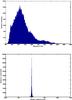 |
Fig. 1 Histogram of simulated dust emission at 857 GHz in pixel domain (top), and wavelet domain at the (bottom). More details about the simulations can be found in Leach (2008). |
3. Sparse component separation: generalized morphological component analysis (GMCA)
3.1. Sparsity for component separation
Sparse priors have been shown to be very useful in regularizing ill-posed inverse problems (Starck et al. 2010). In addition, sparse priors using wavelet bases have been used with success to various signal processing problems in astronomy including denoising, deconvolution, and inpainting (Starck & Murtagh 2006). Like the ICA-based techniques, GMCA aims at solving a blind or semiblind source separation problem. However, GMCA performs in the wavelet domain (Bobin et al. 2008a) to benefit from the sparsity property of the foregrounds in this domain. It is worth mentioning that sparsity has also been used for component separation in fields of research outside astrophysics (Zibulevsky & Pearlmutter 2001; Bobin et al. 2008b, 2009).
In the sequel, we denote the forward wavelet transform by Φ and its backward transform by ΦT. Mathematically speaking, this is a matrix made of wavelet waveforms. One can uniquely decompose each source sj in the wavelet domain as
 where αj are the expansion coefficients of source sj in the wavelet basis. The sparsity of the sources means that most of the entries of αj are equal or very close to zero, and only a few have significant amplitudes. The multichannel data X can be written as
  (12)The objective of GMCA is to seek an unmixing scheme through the estimation of A, which yields the sparsest sources S in the wavelet domain. This is expressed by the following optimization problem written in the augmented Lagrangian form:
 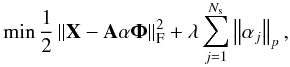 (13)where typically ∥ α ∥ p = ( ∑ k | α [k] | p)1/p. Sparsity is generally enforced for p = 0 which measures the number of non-zero entries of α (or its relaxed convex version with p = 1) and ∥X∥F = (trace(XTX))1/2 is the Frobenius norm. The problem in Eq. (13) is solved in an iterative two-step algorithm such that at each iteration q
Estimation of the S for A fixed to A(q − 1). Solving the problem in Eq. (13) for p = 0 assuming A is fixed to A(q − 1), the sources are estimated as
 where Δλ stands for the hard-thresholding operator with threshold λ. This operator sets all coefficients with amplitudes lower than λ to zero. In practice, the threshold λ is set to be equal to three times the standard deviation of the noise level to exclude noise coefficients. The term A(q − 1) + denotes the Moore pseudo-inverse of the matrix A(q − 1). The Moore pseudo-inverse of some matrix A is defined as (ATA)-1AT.
 Estimation of the A for S fixed to S(q): Updating the mixing matrix assuming that the sources are known and fixed to S(q) is as
3.2. Limitations of GMCA
According to the mixture model underlying GMCA, all the observations are assumed to have the same resolution. However, in most CMB experiments, this assumption does not hold true: the WMAP (resp. Planck) full width at half maximum (FWHM) varies by a factor of about 5 (resp. 7) between the highest resolution and the lowest resolution.
Assuming that the beam is invariant across the sky, the linear mixture model should be substituted with
 where bi stands for the impulse response function of the PSF at channel i. This model can be expressed more by introducing a global multichannel convolution operator ℬ defined so that its restriction to the channel i is equal to a convolution with bi:
  (14)Fully parametric methods have the ability to account for the full mixture. In the family of non-parametric approaches, only blind source separation methods performed in spherical harmonics carefully account for the full mixture model in Eq. (14), where such a model can be simplified naturally (i.e., the convolution operator is diagonalized by the spherical harmonics as in Fourier space for data sampled on regular Euclidean grids). However, this holds true as long as the beam is assumed to be isotropic and invariant across the sky. Extending the data modeling to anisotropic and/or space varying beams can only be made in the pixel domain.
The standard version of GMCA does not model for the different resolutions of the data. For the sake of simplicity, the effect of the beam was neglected during the source separation process. The mixing matrix with GMCA was estimated directly on the data assuming that the linear mixture model is valid. In this setting, the CMB map is evaluated by applying the Moore pseudo-inverse of the estimation mixing matrix to the raw data:
![$$ s = [{\bf A}^+]_{1} {\bf X}, $$](/articles/aa/full_html/2013/02/aa19781-12/aa19781-12-eq112.png) where A + = (ATA)-1AT and the notation [Y] i stands for the ith row of the matrix Y. By convention, matrix elements related to the CMB map have index 1. Neglecting the beam effect implies that the CMB map estimated by GMCA is biased. Hopefully this bias can be computed explicitly by observing that, for each (ℓ,m) in the spherical harmonics domain:
where A + = (ATA)-1AT and the notation [Y] i stands for the ith row of the matrix Y. By convention, matrix elements related to the CMB map have index 1. Neglecting the beam effect implies that the CMB map estimated by GMCA is biased. Hopefully this bias can be computed explicitly by observing that, for each (ℓ,m) in the spherical harmonics domain:
![$$ s_{\ell,m} = \sum_{i=1}^{M} [{\bf A}^+]_{1,i} [{\bf A}]_{i,1} b_{i,\ell} s^\star_{\ell,m} + r, $$](/articles/aa/full_html/2013/02/aa19781-12/aa19781-12-eq118.png) where r is a residual term that models for noise and foregrounds contaminating the estimated CMB. The variable
where r is a residual term that models for noise and foregrounds contaminating the estimated CMB. The variable  stands for the true bias-free CMB in spherical harmonics. By neglecting the residual term, the beam-induced bias can be regarded as a filter in spherical harmonics ℬℓ:
 ![\begin{eqnarray} s_{\ell,m} & \simeq & \left[\sum_{j=1}^M [{\bf A}^+]_{1,j} [{\bf A}]_{j,1} b_{j,\ell} \right] s^\star_{\ell,m} \\ & \simeq & \mathcal{B}_{\ell} s^\star_{\ell,m} \end{eqnarray}](/articles/aa/full_html/2013/02/aa19781-12/aa19781-12-eq122.png) where
where ![\hbox{$\mathcal{B}_{\ell} = \sum_{j=1}^M [{\bf A}^+]_{1,j} [{\bf A}]_{j,1} b_{j,\ell}$}](/articles/aa/full_html/2013/02/aa19781-12/aa19781-12-eq123.png) . The final estimate is computed by inverting the above filter.
. The final estimate is computed by inverting the above filter.
Neglecting the beam effect in the component separation process however has two major drawbacks:
-
Discrepancy with the linear mixture model: the linear mixturemodel does not hold when the data do not share the sameresolution. This very likely leads to a nonoptimal parameterestimation process. According to the linear mixture model, thecontribution of the CMB in the data is the same across frequenciesfor each (ℓ,m), and this contribution is given by the electromagnetic spectrum of the CMB. This is no longer true when the resolution varies from one observation to another and the contribution now varies across ℓ. This means that carrying out component separation from the raw data without accounting for the beam effect should lead to an inaccurate unmixing procedure. The dominant energetic content of the components is mainly concentrated at low frequencies where the beams do not differ too much from each other. At these frequencies, the linear mixture model is a good first-order approximation that may explain the seemingly good performances of GMCA in Leach (2008). However, performances on smaller scales should be enhanced by correctly modeling the beam in the separation process.
-
Noise: following the previous argument, computation of the mixing matrix in GMCA is mainly driven by the low frequency content of the components. However the signal-to-noise ratio (S/N) of the observations highly depends on their resolution; low resolution observations typically have a low S/N at high spatial frequencies. This entails estimating the mixing parameters from the low frequency content for the data but it does not carefully account for the noise contamination on smaller scales, which is likely to lead to low S/N CMB estimates at high ℓ.
We show how GMCA can be modified to solve these problems in the next two sections.
4. GMCA and frequency map resolutions
4.1. Component separation from heterogenous data
The heterogeneity of the data in the separation process can be accounted for in two different ways: the most straightforward technique would consist in adapting GMCA by substituting the data fidelity term in Eq. (13) by the more rigorous expression:  where ℬ represents the beam effect. If this approach has been explored with some success in a different imaging context (Bobin et al. 2009), its high computational cost makes it hard to apply to large-scale CMB data.
The second approach would instead consist in finding ways to apply GMCA to data that share the same resolution. This could be obtained by first converting all the observations to the common desired resolution. However, the beams at low-frequency vanish much faster than at higher frequency and this means that a brute-force deconvolution of the low frequency channels will yield large amplification of the noise. In practice, such a deconvolution is also prohibited by numerical issues. It is important to underline that low resolution channels will mainly add noise to the final estimate at high spatial frequencies (or equivalently high ℓ multipoles in the spherical harmonics domain). Therefore low resolution observations will be the most informative at low frequencies and should be avoided for reconstructing the high frequency content of the CMB map. In the next paragraph, we introduce an elegant strategy for extending GMCA to cope with data involving frequency-dependent beams.
4.2. Multiscale GMCA
A solution to this problem is to adapt the wavelet decomposition for each channel such that the wavelet coefficients  of the M available channels at scale μ do have exactly the same resolution. This can be easily obtained by choosing a specific wavelet function for each channel i (i = 1,··· ,M) such that
  (17)where bi is the beam of the ith channel, btarget the Gaussian beam related to the targeted resolution, and ψμ is the standard wavelet function on scale μ. This approach is closely related to the wavelet-based deconvolution techniques introduced in (Donoho 1995; Khalifa et al. 2003) and called, in the statistical literature, wavelet-vaguelette decomposition. According to this formalism, the decomposition of a function f is defined by
  (18)where Nμ is the number of wavelet scales and Np the number of pixels in the map.
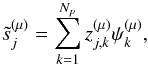
In this paper, we propose extending these ideas to the case of component separation. Replacing the data matrix X by the matrix of wavelet coefficients W ( ), and applying the pseudo inverse of A to W, we get Z = A + W. The quantity
  is now related to the wavelet coefficients of the jth source in the μth wavelet scale at location k. The estimated sources can then be estimated via the following reconstruction formula
  (19)where the notation
  denotes the estimate of the jth source. The reconstruction formula cannot be implemented in practice, because the wavelet coefficients of the ith channel
  on scale μ cannot be calculated when the fraction
  is undefined or numerically unstable. It means that on each wavelet scale μ, only the channels with non-vanishing beams can be used. At the largest wavelet scale, all channels are active, while at the finest wavelet scale, only few channels are active.
We note Cμ the number of channels available for a given resolution level μ, and  the number of wavelet scales that can be used for a given source j. This implies introducing a mixing matrix A(μ) per wavelet scale; this mixing matrix will be evaluated from the Cμ channels available on scale μ. The size of these matrices and the number of sources (limited to the number of channels) vary with μ. For each wavelet resolution level μ, we now have a solution
 (20)where Z(μ) = A(μ) + W(μ), and
  , with i = 1,··· ,Cμ, and μ = 1,··· ,Nμ.
The final solution sj for the jth source is obtained by a simple wavelet reconstruction 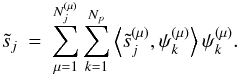 (21)Multiscale GMCA (mGMCA) is similar to a harmonic space method, where we consider one mixing matrix per wavelet band (or frequency band), but unlike SMICA, the mixing matrix is calculated from high-order statistics of wavelet coefficients. Like SMICA, mGMCA can properly take the resolution of the different channels into account but with the paramount advantage that it does not make any assumption on the stationarity of the sources.
4.3. Practical implementation
Though the wavelet-vaguelette source separation method seems a complicated procedure, it can be simplified to a large extent. Indeed, thanks to the linearity of both the beam convolution operator and the wavelet operator, the matrix W(μ) relative to the active channels at resolution level μ can be computed by putting the active maps at the same resolution (which depends on μ) and then computing the same wavelet decomposition on each of them. Once the matrix W(μ) is obtained, one can run the GMCA algorithm to get the mixing matrices A(μ). This can be repeated for each resolution level μ. This way, a CMB map is evaluated for each resolution level, with a number of active channels decreasing with scales. The final solution is then derived by aggregating these solutions in the wavelet space as in Eq. (21).
This procedure leads to not considering in each band the observations that do not have enough resolution; it is noticeable that a similar approach is also used in a recent extension of the ILC (Basak & Delabrouille 2012). Another advantage to this approach is its ability to benefit from the structure of the Healpix format, where different values for the parameter nside can be chosen depending on the resolution level, which speeds up the computation time.
As an illustration, we give a possible parameterization of mGMCA for Planck data. In this case, we have nine channels from 30 to 857 GHz, with a resolution that goes roughly from 33 arcmin to 5 arcmin. We have therefore considered five resolution levels, with a number of active channels varying from nine to five (see Table 1). The corresponding wavelet filters are depicted in Fig. 2.
Example of resolution levels to use in mGMCA, with the number of active channels per resolution level.
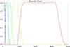 |
Fig. 2 Wavelet filters in the spherical harmonics domain. Abscissa: spherical harmonics multipoles ℓ. Ordinate: amplitude of the wavelet filters. |
However, the underlying modeling of mGMCA does not allow for a precise separation of components with spectral variations. The next section shows that the spatial variation of the matrix can also be taken into account when using a partitioning of the wavelet scales.
5. GMCA and spatially variant mixing matrix
5.1. A refined modeling to get closer to astrophysics
As emphasized in the introduction, the complexity of CMB data makes it very hard to fully model for all the physical phenomena with a simple linear mixture model. The linear mixture model used so far in most component separation methods assumes that: i) the number of components is limited to the total number of observations; and ii) explicitly that the emissivity of the component is space invariant (i.e. the mixing matrix does not vary from one pixel to another). Unfortunately, these assumptions are not verified by common CMB data. The components one observes between 30 GHz and 857 GHz include the CMB, Sunyaev Zel’Dovich effect, free-free, synchrotron, CIB, anomalous dust and dust emissions as well as IR and radio sources the number of which largely exceeds the number of observations provided by Planck. From the current knowledge in astrophysics, some of these components can be approximated quite accurately with space-invariant emissivity, which is the case for the CMB, SZ effect, free-free and synchrotron emission. The dust emissions provide a very important, if not dominant, contribution in high frequency channels. These channels have the highest spatial resolution (typ. 5 to 10 arcmin); modeling for such a component should thus be of utmost importance for a high-resolution estimate of the CMB map. However modeling dust emission is a strenuous problem. Indeed, contrary to well-characterized foreground emissions such as free-free or synchrotron, most component separation models do not satisfactorily model this contribution. As an example, the gray-body dust model, known as one of the most accurate dust models, involves two parameters: a spectral index and temperature varying across pixels. These remarks imply that the linear mixture model does not allow for enough degrees of freedom to fully capture the complexity of CMB data in the frequency range observed by most CMB surveys like Planck. In the following, we focus on extending this model to account for spatially variant spectra.
5.2. Multiscale local mixture model
The global mixture model used by most component separation methods do not allow for enough degrees of freedom to naturally capture scale/space-dependent astrophysical phenomena. The scale-dependance of the analysis naturally arises from the mGMCA formalism, and localization requires decomposing each wavelet scale into patches. It is worth mentioning that localizing the estimation of the CMB has also been proposed within the ILC framework (Delabrouille et al. 2009) to analyze WMAP map data. N-ILC consists in: i) decomposing each wavelet scale into patches with a scale-dependent size; and ii) performing ILC on each patch independently. However, the spectral behavior of many components is not expected to change dramatically from one patch to its neighbor, but such an independent processing each on patch may not be optimal.
For this purpose, we have extended the mixture model to a multiscale local mixture model. In such modeling, each location of the sky in each wavelet scale is analyzed several times with different patch sizes which allows the best parameters to be locally selected.
Before going any further, we first recall some useful notations. If X denotes the data, we denote the matrix composed of the μth wavelet scale of the data X by W(μ). In what follows, the indexing W(μ) [k] denotes the square patch of size p centered on pixel k. Following the multiscale local model, a patch-based representation of the data on scale μ and location k is modeled as ![\begin{equation} \label{eq:mlml} {\bf W}^{(\mu)}[k] = {\bf A}^{(\mu)}[k] {\bf S}^{(\mu)} [k] + {\bf N}^{(\mu)}[k]. \end{equation}](/articles/aa/full_html/2013/02/aa19781-12/aa19781-12-eq163.png) (22)A direct extension of mGMCA to solve this problem would simply amount to applying GMCA independently to each patch at location k and on each scale μ. However, this approach would suffer from certain drawbacks assuming that some “optimal” patch size at each scale μ is known and fixed in advance. However, fixing a priori the patch size is a very strong constraint because the appropriate patch size should be space-dependent as well and may vary from one region to another.
(22)A direct extension of mGMCA to solve this problem would simply amount to applying GMCA independently to each patch at location k and on each scale μ. However, this approach would suffer from certain drawbacks assuming that some “optimal” patch size at each scale μ is known and fixed in advance. However, fixing a priori the patch size is a very strong constraint because the appropriate patch size should be space-dependent as well and may vary from one region to another.
This suggests that a trade-off should be made between small/large patches which would balance between statistical consistency (large patches) and adaptivity (small patches). This indicates that the choice of the patch size should be adaptive and dependent on the local content of the data. Inspired by best basis techniques in multiscale signal analysis, an elegant way to alleviate this pitfall is to perform GMCA on each wavelet scale μ with various patch sizes in a quadtree decomposition. In a nutshell, GMCA is first performed on the full field to obtain a first estimator of the mixing matrix denoted by ![\hbox{${\bf A}_2^{(\mu)}[k]$}](/articles/aa/full_html/2013/02/aa19781-12/aa19781-12-eq164.png) in Fig. 3. The field is further decomposed into four identical non overlapping patches on which GMCA is applied to provide a set of mixing matrices denoted
in Fig. 3. The field is further decomposed into four identical non overlapping patches on which GMCA is applied to provide a set of mixing matrices denoted ![\hbox{${\bf A}_1^{(\mu)}[k]$}](/articles/aa/full_html/2013/02/aa19781-12/aa19781-12-eq165.png) in the figure. The process is iterated until the patch is equal to the desired patch size pμ. The number of analysis levels is equal to Lμ. Interestingly, because the same area of the sky is analyzed on different mixture scales (i.e. patch sizes), it makes it possible to choose the “optimal” patch size from the different estimates obtained for l = 0,...,Lμ afterwards. It therefore allows for more degrees of freedom in selecting an adapted patch size at each location. An exhaustive description of the parameter selection strategy is given in Appendix A.
in the figure. The process is iterated until the patch is equal to the desired patch size pμ. The number of analysis levels is equal to Lμ. Interestingly, because the same area of the sky is analyzed on different mixture scales (i.e. patch sizes), it makes it possible to choose the “optimal” patch size from the different estimates obtained for l = 0,...,Lμ afterwards. It therefore allows for more degrees of freedom in selecting an adapted patch size at each location. An exhaustive description of the parameter selection strategy is given in Appendix A.
5.3. The L-GMCA algorithm
The local GMCA (L-GMCA) algorithm can be described as follows:
| 1. Compute the wavelet decomposition of the data. |
| 2. For each wavelet scale μ = 1,··· ,Nμ: |
| 2.1 Put the Cμ active channels to the same targeted |
| resolution |
| 2.2 For each local k: |
| 2.2.1 – Compute a set of mixing matrices at different |
| patch sizes (Lμ levels of analysis) |
| 2.2.2 – Select the optimal mixing matrix |
| 2.2.3 – Compute the CMB map estimate at scale μ |
| and location k. |
| 3. Reconstruct the CMB map following Eq. (21). |
Once the mixing matrices are estimated with L-GMCA (steps 2.2.1 and 2.2.2 of the algorithm), estimating the CMB map requires performing both a wavelet-vaguelette decomposition and a weighting of the wavelet coefficient of the multifrequency data on each wavelet scale according to the pseudo-inverse values of the estimated local mixing matrix. This sequence of operations is particularly computer intensive for high resolution data (e.g. Npix ≃ 50 million pixels for Planck data for each of the 9 frequency maps), requiring for each resolution level and each channel two back and forth spherical harmonic transforms (of asymptotic complexity Npix3/2) followed by two wavelet transforms for each HEALPix face (of asymptotic complexity Npixlog (Npix)), and a weighting of each coefficient map on each scale and each resolution level (of asymptotic complexity Npix). This should be multiplied by the number of Monte-Carlo simulations. We developed a C++ parallelized program using OpenMP. As an illustration of how crucial computer speed might be, on a shared-memory multiprocessor system containing eight Six-Core AMD Opteron(tm) running at 2.4 GHz, recovering the CMB map from one Monte-Carlo simulation takes about nine minutes when 24 processors are used.
 |
Fig. 3 Multichannel quadtree decomposition to display the tree-based decomposition of the multichannel data W(μ). A sequence of mixing matrices is estimated on patches with dyadically decreasing size. Large sized patches are used as a warm startup for the estimation process on smaller patches. |
6. Experiments
6.1. Simulations and comparisons
In early 2013, the finest – low noise, high resolution – CMB data will be Planck data. Therefore, in this section, we propose evaluating the performances of the proposed approach with simulated Planck data. To the best of our knowledge, the only publicly available full-sky simulated Planck data are the dataset used to evaluate preliminary performances of various CMB map estimation techniques in 2008. This pre launch study has been published in Leach (2008). In the sequel, numerical experiments will be performed using exactly the same Planck simulated dataset. Before going deeper into the description of the numerical results, the next paragraphs clarify the astrophysical content of the simulation, as well as the evaluation protocol we opted for.
Some words about the simulations:
the Planck-like dataset described in Leach (2008) has been simulated using an early version of the Planck Sky Model (PSM) developed by J. Delabrouille and collaborators2 in Delabrouille (2012). In 2008, the PSM included most astrophysical signals and foregrounds, as well as simulated instrumental noise and beams. In detail, the simulations were obtained as follows.
-
Frequency channels: the simulated data are comprised of the 9 LFI and HFI channels at frequency 33,44,70,100,143,217,353,545,857 GHz. The frequency-dependent beams are perfect isotropic Gaussian PSF with FWHM ranging from 5 arcmin at 217,353,545,857 GHz to 33 arcmin at 33 GHz. Real data differ from the model since the scanning strategy adopted by full-sky surveys, such as WMAP or Planck is likely to produce non-isotropic and spatially varying beams that are more elongated in the scanning direction.
-
Instrumental noise: in full-sky surveys, the sky coverage is generally not uniform, because some areas are more often observed than others. To some extent, this entails that the instrumental noise variance is not homogenous as well. The noise statistics (i.e. noise variance map for each frequency channel) are assumed to be known accurately. These statistics are consistent with the Planck noise variance maps (Leach 2008). In statistical signal processing, this kind of statistical process is better known as heteroscedastic noise. A second effect of the scanning strategy is the correlation of the noise along the scanning direction. In the sequel, simulations account for the heterogeneity of the noise but noise samples are assumed to be uncorrelated.
-
Cosmic microwave background: the CMB map is a correlated random Gaussian realization entirely characterized by its power spectrum. In the simulations, the CMB power spectrum is identical to that of WMAP. Higher order multipoles are based on a WMAP best-fit power spectrum at high ℓ. The simulated CMB is Gaussian, and no non-Gaussianity (e.g. lensing, ISW, fNL) has been added. This will allow for non Gaussianity tests under the null assumption in the sequel.
-
Dust emissions: the galactic dust emissions is composed of two distinct dust emissions: thermal dust and spinning dust (a.k.a. anomalous microwave emission). Thermal dust is modeled with the Finkbeiner model (Finkbeiner et al. 1999), which assumes that two hot/cold dust populations contribute to the signal in each pixel. The emission law of thermal dust varies across the sky.
-
Synchrotron emission: the synchrotron emission, as simulated by the PSM, is an extrapolation of the Haslam 408 MHz map (Haslam et al. 1982). The emission law of the synchrotron emission is an exact power law with a spatially varying spectral index.
-
Free-free emission: the spatial geometry of free-free emission is inspired by the Hα map built from the SHASSA and WHAM surveys. The emission law is a perfect power law with a fixed spectral index.
-
Point sources: infrared and radio sources were added based on existing catalogs at that time. In the following, the brightest point sources is masked prior to the evaluation results.
-
Sunyaev Zel’Dovich effect: thermal SZ is modeled in the simulations.
Comparison protocol:
in 2008, most of the estimated CMB maps used for comparisons were quite heterogenous by not necessarily sharing the same beams. As a consequence, precise and quantitative evaluations were very hard to carry out. However, with the exception of GMCA3, none of the codes used to estimate CMB maps in Leach (2008) is publicly available. The major objective of this paper has been to evaluate the impact of the local and multiscale mixture model, as well as the sparsity-based component separation technique we introduced in this paper. Since WMAP, ILC and its extensions (Delabrouille et al. 2009; Remazeilles et al. 2011) are very popular in the astrophysics community. Like most component separation techniques in cosmology, ILC relies on second order statistics (more precisely, χ2 minimization) to estimate the CMB map. For this reason, we first chose to compare two different separation methods: GMCA (based on sparsity) and ILC (based on second order statistics). Furthermore, we believe that one of the contributions of this paper is the use of the local modeling in the wavelet domain. We also evaluate the performances of methods along with a global mixture model (the corresponding methods will be ILC and GMCA), as well as with the local mixture model in wavelets (L-GMCA).
Parameters used in local and multiscale sky model.
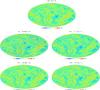 |
Fig. 4 Input (top) and estimated CMB maps in mK. |
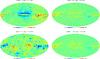 |
Fig. 5 Residual CMB maps. These maps are defined as the difference between the estimated maps and the input CMB map. Units in mK. |
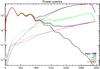 |
Fig. 6 Power spectrum of the maps. The solid black line is power spectrum of the input CMB map at the resolution of 5 arcmin. Abscissa: spherical harmonics multipoles ℓ. Ordinate: power spectra value – units in ℓ(ℓ + 1)Cℓ/(2π)mK2 |
The local and multiscale model requires defining four parameters: i) the number of sources is set to be equal to the number of channels; ii) the number of wavelet scales; iii) the number of quad-tree decomposition levels Lμ; and iv) the nominal patch size pμ. All these parameters are given in Table 2. There is no automatic strategy for optimally selecting these parameters. We would like to point out that a non-exhaustive series of experiments; the particular choice of Table 2 turned out to provide lower power spectrum bias, especially at high ℓ. NILC (Needlet-ILC) has also been performed (Delabrouille et al. 2009; Basak & Delabrouille 2012).
In the sequel, a 92% common mask, which preserves a very large part of the sky, has been defined as the union of a small galactic mask and a point source mask that has been derived from the brightest point sources.
6.1.1. CMB map estimation
In this paragraph, we mainly focus on the quality of the estimation of the full-sky CMB map. Figure 4 displays the input CMB at a resolution of 5 arcmin on top and the maps we obtained by performing ILC, GMCA, NILC, and L-GMCA. More interestingly, Fig. 5 shows the residual maps we defined as the difference between the estimated maps and the input CMB map at 5 arcmin. These error maps have been filtered further at the resolution of 45 arcmin to filter out the noise contamination that dominates at high frequency, which allows the low frequency foreground residuals which remain in the final estimates to better unveiled. The ILC residual map (top-left picture) clearly exhibits large-scale features which are reminiscent of the synchrotron emission (negative bulb centered about the galactic center), as well as free-free emissions relics (well-known positive free-free on the right of the residual map) and dust emission. The NILC residual show significant large scale “blobby” effects that may be related to the use of the needlet filters used for the analysis rather than more space-localized wavelet filters. Visually, GMCA and L-GMCA seem to have similar remaining foreground contamination, which is evocative of dust emission.
Figure 6 shows the power spectra of the CMB maps. These spectra were computed from the noisy CMB maps. Therefore, on intermediate and small scales (ℓ > 500.) the observed bias mainly comes from the contribution of noise as shown by the dotted lines. In this figure, the differences between the different methods highlight their respective noise contamination level. Global methods, and especially ILC, exhibit a large noise level at high ℓ, but these methods do not account for the beam variation across channels. Therefore, ILC and GMCA are mainly sensitive to the largest scales and do not carefully deal with noise contamination on smaller scales. Space/scale localized approaches like L-GMCA and NILC have lower noise contamination with only slight differences between them. It is remarkable that, if NILC is expected to exhibit low noise contamination (i.e. it relies on the second order statistics of the data), L-GMCA is also designed well to provide low noise contamination levels.
6.2. Foreground contamination
An accurate measure of foreground contamination is the cross power spectrum between the residual map and the maps of the input foregrounds. We evaluated the cross power spectra of foreground templates used in the simulations with the error maps defined by the difference between the input CMB map (a.k.a. the true CMB map) and estimated CMB maps. These cross power spectra have been performed with synchrotron emission in Fig. 7, free-free in Fig. 8, dust emission in Fig. 9, and SZ effect in Fig. 10. The same study has been carried out with synchrotron but it did not show significant differences between the four methods.
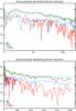 |
Fig. 7 Cross-power spectra of the estimated CMB map with the synchrotron template. |
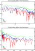 |
Fig. 8 Cross-power spectra of the estimated CMB map with the free-free template. |
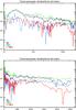 |
Fig. 9 Cross-power spectra of the estimated CMB map with the thermal dust template. |
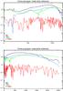 |
Fig. 10 Cross-power spectra of the estimated CMB map with the SZ template. |
The conclusion we can draw from this cross-correlation study are the following:
-
1.
Accurately accounting for the beams: the heterogeneity of thedata (i.e. the beam varies across frequencies) is better accountedfor. As explained in Sect. 4.1, an inaccurate model-ing for the beams increases the complexity of the mixtures. Evenif the emission law of a given component is spatially invariant, thevariability of the beam across frequencies make this emissionlaw variant across multipoles in spherical harmonics. This is es-pecially striking for the SZ component in Fig. 10,because its emission law is known exactly and fixed in bothGMCA and L-GMCA. However, the two methods show radi-cally different cross-correlation with the SZ template. Fixingthe SZ emission does not guarantee that its contamination levelvanishes if the beam is not properly taken into account. In these simulations, the electromagnetic spectrum does not vary across the sky. Assuming the beam does not change across frequencies, its estimation should be made efficiently on all scales with methods based on global mixture models. However, as shown in Fig. 8, GMCA and ILC exhibit a high level of free-free contamination; especially for ℓ > 100 in the case of ILC. Again, the ability of the proposed modeling to account for heterogeneous beams allows for a lower free-free contamination level.
-
2.
More flexible modeling: whether NILC or L-GMCA, the local and multiscale mixture model we introduced in this paper allows for more degrees of freedom to better analyze complicatedly mixed components. In all the correlations computed so far, the techniques based on this modeling have outperformed the methods using the simple (but commonly used) global linear mixture model. This is particularly the case for synchrotron, free-free and dust emissions in Figs. 7–9, where methods based on the local/multiscale model exhibit lower foreground contamination.
-
3.
Sparsity versus second-order statistics: the strong SZ contamination of ILC-based methods enlightens the low efficiency of second-order statistics to capture non-Gaussian foregrounds. Conversely, sparsity-based component separation techniques are much more effective at separating the CMB and non Gaussian contaminants. The sensitivity of sparsity to higher order statistics is very likely at the origin of the lower synchrotron and dust contamination of L-GMCA for ℓ > 1000.
6.3. Non Gaussian contamination
The CMB we used in these simulations is a perfect correlated Gaussian random field; more precisely, it contains no trace of non-Gaussianity regardless of whether it is ISW, lensing, or fNL. CMB non-gaussianities will evidently come from spurious foreground contaminations. In this paragraph, we propose evaluating the level of (non) Gaussianity of the estimated CMB. Since the CMB is perfectly Gaussian in these simulations, such a study will give a different measure of the contamination level.
Common non-Gaussianity tests consist in computing the higher order statistics of the estimated residual maps in the wavelet domain (Starck & Murtagh 2006). The aim of this study is to give a different way to measure foreground contamination. We instead opted for evaluating of the non-Gaussianity (NG) level of the residual maps instead of the CMB. This has the crucial advantage of providing a contamination level measure insensitive to CMB fluctuations. For this purpose, several statistical tests were performed: the kurtosis (i.e. statistics of order 4) is calculated on the 5 first wavelet scales of the residual maps. These results are shown in the top pictures of Fig. 11. The residual map then contains the foreground residuals as well as the remaining instrumental noise that contaminates the estimated CMB maps. If one wants to quantify the level of foreground residuals, noise is the only statistical component. The significance of the results is then evaluated through 25 independent Monte-Carlo simulations of noise maps. The dotted lines in Fig. 11 are computed as the 3σ confidence interval which we derived from these simulations. Except on very large scale (ℓ < 200), these two measures of non-Gaussianities draw very similar conclusions: i) on the first wavelet scale, all the three methods are likely to be compatible with a Gaussian contamination, and this mainly comes from the preeminence of noise in this range; ii) the sparsity – based separation criterion used in L-GMCA yields lower NG levels in the scales 2 to 4 (i.e. 200 ≤ ℓ ≤ 1600). At large scale, L-GMCA has a lower kurtosis value. At that stage, massive simulations of all the components (and not only noise) would be mandatory to precisely evaluate the performances of these methods at low ℓ. The lower graph of Fig. 11 features the value of the kurtosis on fixed wavelet scales but in different equiangular bands of latitude. By convention, the data were in galactic coordinates where latitude 0 corresponds to the galactic plane. From these pictures, L-GMCA is likely to be less contaminated than the three other residual maps. More significantly, GMCA exhibits lower NG contamination at all latitudes on scales 2 to 4. This highlightens the role of GMCA and more precisely the use of sparsity to better extract non-Gaussian sources. It is very likely that the second order statistics used as a separation criterion in ILC is less sensitive than sparsity to separate foregrounds. This unveils the positive impact of the local and multiscale model, together with a sparsity-based separation criterion as used in L-GMCA.
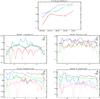 |
Fig. 11 Kurtosis of the estimated CMB maps in the wavelet domain. Top: per wavelet scale. Per latitude – top-left panel: first wavelet scale. Top-right panel: second wavelet scale. Bottom-left panel: third wavelet scale. Bottom-right panel: fourth wavelet scale. Dashed lines are 3σ confidence interval computed from 25 random noise realizations. |
Software
Source separation techniques used in cosmology and more precisely for CMB map estimation are generally high-end methods that are seldom publicly shared and available online4.
7. Conclusion
The estimation of a high-precision CMB map featuring low noise and low foreground contamination is crucial for the astrophysical community. This problem is customarily tackled in the framework of component separation. As for any estimation problem, accurate modeling of the data is essential. However, a close look at the astrophysical phenonema in play in the CMB data, such as WMAP or Planck, reveals that the linear mixture model used so far by common component separation methods in cosmology does not hold. First, the variation in the beam across scale is seldom accounted for, which highly limits the performances of these component separation methods, especially on small scales. More important, the linear mixture model does not afford enough degrees of freedom to precisely capture the complexity of the data, including the variability across space of the emission law for some of the components of interest.
To alleviate these limitations, this paper introduces a new modeling of the components’ mixtures using a multiscale and local decomposition of the data in the wavelet domain. We introduced a novel sparsity-based coined L-GMCA, which profits from the proposed local/multiscale mixture model. In the proposed framework, wavelet-based multiscale analysis allows for precise modeling of the beam evolution across channels. Capturing the variations across pixels of the emissivity of components is carried out by partitioning each wavelet scale with adaptive patch sizes. Extensive numerical experiments have been carried out to show that the proposed modeling and separation technique provides a clean, low-foreground CMB map estimate. More precisely, we showed that the local and multiscale modeling allows for improved separation results even when it is used with separation techniques as different as ILC and GMCA. Additionally, the numerical experiments brings out the dramatic positive impact of the use of sparsity in L-GMCA to provide less galactic foreground contamination, as well as significantly lower non-Gaussianity levels.
GMCA is part of the ISAP toolbox: http://jstarck.free.fr/isap.html
For more details about the PSM, we invite the reader to visit the PSM website: http://www.apc.univ-paris7.fr/~delabrou/PSM/psm.html
GMCA is available at this address: http://jstarck.free.fr/isap.html
The L-GMCA code will be made publicly available at http://www.cosmostat.org/lgmca.html
Acknowledgments
This work was supported by the French National Agency for Research (ANR -08-EMER-009-01) and the European Research Council grant SparseAstro (ERC-228261).
References
- Aumont, J., & Macías-Pérez, J. F. 2007, MNRAS, 376, 739 [NASA ADS] [CrossRef] [Google Scholar]
- Basak, S., & Delabrouille, J. 2012, MNRAS, 419, 1163 [NASA ADS] [CrossRef] [Google Scholar]
- Bedini, L., Herranz, D., Salerno, E., et al. 2005, EURASIP J. Appl. Signal Proc., 2005, 2400 [Google Scholar]
- Bennett, C. L., Halpern, M., Hinshaw, G., et al. 2003a, ApJS, 148, 1 [NASA ADS] [CrossRef] [Google Scholar]
- Bennett, C. L., Hill, R. S., Hinshaw, G., et al. 2003b, ApJS, 148, 97 [NASA ADS] [CrossRef] [Google Scholar]
- Bobin, J., Starck, J.-L., Fadili, M. J., & Moudden, Y. 2007, IEEE Transactions on Image Processing, 16, 2662 [Google Scholar]
- Bobin, J., Moudden, Y., Starck, J. L., Fadili, M., & Aghanim, N. 2008a, Stat. Meth., 5, 307 [NASA ADS] [CrossRef] [Google Scholar]
- Bobin, J., Starck, J.-L., Moudden, Y., & Fadili, M. J. 2008b, Advances in Imaging and Electron Physics, 152, 221 [CrossRef] [Google Scholar]
- Bobin, J., Moudden, Y., Starck, J.-L., & Fadili, J. 2009, in Wavelets: Applications in Signal and Image Processing XIII, eds. V. K. Goyal, M. Papadakis, & D. Van De Ville, Proc. SPIE, 7446 [Google Scholar]
- Bouchet, F. R., Prunet, S., & Sethi, S. 1999, MNRAS, 302, 663 [NASA ADS] [CrossRef] [Google Scholar]
- Bouchet, R., & Gispert, R. 1999, New Astron., 4 [Google Scholar]
- Comon, P., & Jutten, C. 2010, Handbook of blind source separation (Academic Press) [Google Scholar]
- Delabrouille, J., Cardoso, J.-F., & Patanchon, G. 2003, MNRAS, 346, 1089 [NASA ADS] [CrossRef] [Google Scholar]
- Delabrouille, J., Cardoso, J.-F., Jeune, M. L., et al. 2009, A&A, 493, 835 [NASA ADS] [CrossRef] [EDP Sciences] [Google Scholar]
- Delabrouille, J., Belin, J.-B., Betoule, M., et al. 2012, A&A, submitted [arXiv:1207.3675] [Google Scholar]
- Dickinson, C., Davies, R., & Davis, R. 2003, MNRAS, 341 [Google Scholar]
- Donoho, D. 1995, Appl. Computat. Harmonic Analys., 2, 101 [Google Scholar]
- Dunkley, J., Amblard, A., Baccigalupi, C., et al. 2009, in AIP Conf. Ser. 1141, eds. S. Dodelson, D. Baumann, A. Cooray, et al., 222 [Google Scholar]
- Eriksen, H. K., Banday, A. J., Gorski, K. M., & Lilje, P. B. 2004, ApJ, 612 [Google Scholar]
- Eriksen, H. K., Jewell, J. B., Dickinson, C., et al. 2008, ApJ, 676, 10 [NASA ADS] [CrossRef] [Google Scholar]
- Fernández-Cobos, R., Vielva, P., Barreiro, R. B., & Martínez-González, E. 2012, MNRAS, 420, 2162 [NASA ADS] [CrossRef] [Google Scholar]
- Finkbeiner, D., Davis, M., & Schlegel, D. 1999, ApJ, 524 [Google Scholar]
- Fixsen, D. J., Dwek, E., Mather, J. C., Bennett, C. L., & Shafer, R. A. 1998, ApJ, 508, 123 [NASA ADS] [CrossRef] [Google Scholar]
- Gorski, K., Hivon, E., Banday, A. J., et al. 2005, ApJ, 622 [Google Scholar]
- Haslam, C., Salter, C., Stoffel, H., & Wilson, W. E. 1982, A&AS, 47, 1 [NASA ADS] [Google Scholar]
- Hastie, T., Tibshirani, R., & Friedman, J. 2009, The Elements of Statistical Learning: Data Mining, Inference, and Prediction (Springer) [Google Scholar]
- Hobson, M. P., Jones, A. W., & Lasenby, A. N. 1999, MNRAS, 309, 125 [NASA ADS] [CrossRef] [Google Scholar]
- Hurier, G., Hildebrandt, S., & Macias-Perez, J. 2010 [arXiv:1007.1149] [Google Scholar]
- Hyvarinen, A., Karhunen, J., & Oja, E. 2001, Independent Component Analysis (New York: J. Wiley) [Google Scholar]
- Kay, S. 1993, Fundamentals Of Statistical Signal Processing: Estimation Theory (Prentice Hall) [Google Scholar]
- Khalifa, J., Mallat, S., & Rougé, B. 2003, IEEE Transactions on Image Processing, 12, 446 [Google Scholar]
- Leach, S. 2008, A&A, 491, 597 [NASA ADS] [CrossRef] [EDP Sciences] [Google Scholar]
- Marinucci, D., Pietrobon, D., Balbi, A., et al. 2008, MNRAS, 383, 539 [NASA ADS] [CrossRef] [Google Scholar]
- Miville-Deschênes, M.-A., Lagache, G., Boulanger, F., & Puget, J.-L. 2007, A&A, 469, 595 [NASA ADS] [CrossRef] [EDP Sciences] [Google Scholar]
- Moudden, Y., Cardoso, J.-F., Starck, J.-L., & Delabrouille, J. 2005, EURASIP J. Appl. Signal Processing, 2005, 2437 [Google Scholar]
- Planck Collaboration 2006, Planck: The scientific programme (ESA) [Google Scholar]
- Planck Collaboration 2011a, A&A, 536, A19 [NASA ADS] [CrossRef] [EDP Sciences] [Google Scholar]
- Planck Collaboration 2011b, A&A, 536, A7 [NASA ADS] [CrossRef] [EDP Sciences] [Google Scholar]
- Planck Collaboration 2011c, A&A, 536, A20 [NASA ADS] [CrossRef] [EDP Sciences] [Google Scholar]
- Remazeilles, M., Delabrouille, J., & Cardoso, J.-F. 2011, MNRAS, 410, 2481 [NASA ADS] [CrossRef] [Google Scholar]
- Starck, J.-L., & Murtagh, F. 2006, Astronomical Image and Data Analysis, 2nd edn. (Springer) [Google Scholar]
- Starck, J.-L., Moudden, Y., Abrial, P., & Nguyen, M. 2006, A&A, 446, 1191 [NASA ADS] [CrossRef] [EDP Sciences] [Google Scholar]
- Starck, J.-L., Murtagh, F., & Fadili, M. 2010, Sparse Image and Signal Processing (Cambridge University Press) [Google Scholar]
- Stolyarov, V., Hobson, M. P., Lasenby, A. N., & Barreiro, R. B. 2005, MNRAS, 357, 145 [NASA ADS] [CrossRef] [Google Scholar]
- Sunyaev, R. A., & Zeldovich, Y. B. 1970, Astrophys. Space Sci., 7, 3 [Google Scholar]
- Zibulevsky, M., & Pearlmutter, B. 2001, Neural Computation, 13, 863 [Google Scholar]
Appendix A: Multiscale local mixture model
Before going further into the description of the method, principles of the multichannel quadtree decomposition and notations have to be discussed. In multiscale image analysis, quadtree decomposition amounts to decomposing each wavelet scale in patches with dyadic sizes starting from the original field itself and sequentially subdivide each patch to four. To our knowledge, this multiscale analysis procedure has never been extended to analyze multichannel data in a source separation framework. In this specific context, such an extension consists in estimating the mixture parameters (i.e. the mixing matrix A and the sources S) on each scale μ on patches with various patch sizes starting from large patches of size 2Lμpμ to smaller patches of size pμ. The parameter Lμ denotes the number of decomposition levels or subdivisions in which the estimation of the mixture parameters is carried out. Figure 3 clearly illustrates the principle of the decomposition where the analysis (i.e. estimation of the mixing matrices) is first performed on the largest patch size allowed 2Lμpμ: ![\hbox{${\bf W}^{(\mu)}_{L_\mu}[k]$}](/articles/aa/full_html/2013/02/aa19781-12/aa19781-12-eq196.png) . In the next step, the patch is divided into 4 non overlapping patches of size 2Lμ − 1pμ on which the parameters estimation is carried out. The same process is performed until the final patch size pμ is attained. The notation we use in the sequel is the following:
. In the next step, the patch is divided into 4 non overlapping patches of size 2Lμ − 1pμ on which the parameters estimation is carried out. The same process is performed until the final patch size pμ is attained. The notation we use in the sequel is the following:
-
Multichannel patch
![\hbox{${\bf W}^{(\mu)}_l[k]$}](/articles/aa/full_html/2013/02/aa19781-12/aa19781-12-eq198.png) : is the concatenation of Nμ frequency patches of size 2lpμ × 2lpμ as defined in Fig. 3 centered on pixel k. We invite the reader to notice that the three indices of the notations
: is the concatenation of Nμ frequency patches of size 2lpμ × 2lpμ as defined in Fig. 3 centered on pixel k. We invite the reader to notice that the three indices of the notations ![\hbox{${\bf W}_l^{(\mu)}[k]$}](/articles/aa/full_html/2013/02/aa19781-12/aa19781-12-eq200.png) underlines the dependence of this variable on the: i) the pixel at which the analysis is carried out; ii) the wavelet scale μ and the quadtree decomposition level l.
underlines the dependence of this variable on the: i) the pixel at which the analysis is carried out; ii) the wavelet scale μ and the quadtree decomposition level l. -
Multichannel patch
![\hbox{${\bf A}^{(\mu)}_l[k]$}](/articles/aa/full_html/2013/02/aa19781-12/aa19781-12-eq202.png) : mixing matrix estimated from the multichannel patch .
: mixing matrix estimated from the multichannel patch .
Interestingly, since the same area of the sky is analyzed on different mixture scales (i.e. patch sizes), it is possible to choose afterwards the “optimal” patch size from the different estimates obtained for l = 0,··· ,Lμ. It therefore allows for more degrees of freedom in selecting an adapted patch size at each location. Full-sky CMB data (e.g. WMAP, Planck) are generally sampled on the Healpix sampling grid (Gorski et al. 2005). For the sake of simplicity and computational efficiency, the most straightforward way to decompose an Healpix map into patches is to decompose each Healpix face.
Choosing the “optimal” patch decomposition
For each patch location k, L-GMCA provides a sequence of parameters or more specifically mixing matrices computed on different mixtures scales: ![\hbox{$\left\{ {\bf A}^{(\mu)}_l[k] \right\}_{l=0,\cdots,L_\mu}$}](/articles/aa/full_html/2013/02/aa19781-12/aa19781-12-eq204.png) . These mixing matrices have been computed from patches of increasing sizes; this entails they offer different views of the data in the neighborhood of pixel k. As emphasized in the previous section, this allows for extra flexibility in choosing adapted local parameters: i) mixing matrices estimated from larger areas will be more adapted to stationary areas; ii) mixing matrices evaluated from local patches analysis are well-suited to better capturing local variations in the foreground emissivity. The difficulty now mainly consists in defining a strategy to select the optimal local estimator of the mixing matrix (i.e. optimal amongst the set of available estimators).
. These mixing matrices have been computed from patches of increasing sizes; this entails they offer different views of the data in the neighborhood of pixel k. As emphasized in the previous section, this allows for extra flexibility in choosing adapted local parameters: i) mixing matrices estimated from larger areas will be more adapted to stationary areas; ii) mixing matrices evaluated from local patches analysis are well-suited to better capturing local variations in the foreground emissivity. The difficulty now mainly consists in defining a strategy to select the optimal local estimator of the mixing matrix (i.e. optimal amongst the set of available estimators).
First, it has to be noticed that in the framework of GMCA and similarly in L-GMCA, once the mixing matrices are estimated, the final estimate of the components are computed by applying the Moore pseudo-inverse of the mixing matrix to the data:
 This way the sources linearly depend on the original data Wμ; this is particularly important for controlling error propagation in the final CMB map estimate.
Distinguishing between the available mixing matrices at location k amounts to defining a criterion sensitive the local misestimation of the CMB map. From the sequences of available mixing matrices ![\hbox{$\{{\bf A}^{(\mu)}_l[k]\}_{l=0,\cdots,L_\mu}$}](/articles/aa/full_html/2013/02/aa19781-12/aa19781-12-eq207.png) , one can compute a sequence of various local CMB map estimates about pixel k at the level of the smallest patch of size pμ. These estimates are computed by applying the pseudo-inverse of the different matrices to the smallest data patch about pixel k,
, one can compute a sequence of various local CMB map estimates about pixel k at the level of the smallest patch of size pμ. These estimates are computed by applying the pseudo-inverse of the different matrices to the smallest data patch about pixel k, ![\hbox{${\bf W}^{(\mu)}_{l=0}[k]$}](/articles/aa/full_html/2013/02/aa19781-12/aa19781-12-eq208.png) :
:
![$$ {\bf S}^{(\mu)}_l[k] = {{\bf A}_l^{(\mu)}}^+ {\bf W}_{l=0}^{(\mu)}[k]. $$](/articles/aa/full_html/2013/02/aa19781-12/aa19781-12-eq209.png) Quite naturally, the optimal mixing matrix amongst the available estimators
Quite naturally, the optimal mixing matrix amongst the available estimators ![\hbox{$\left\{ {\bf A}_l^{(\mu)}[k] \right\}_{l=0,\cdots,L_\mu}$}](/articles/aa/full_html/2013/02/aa19781-12/aa19781-12-eq210.png) should be chosen such that the estimated CMB is the least contaminated possible. Here contamination is taken in the wide sense: foreground and noise. One remarkable property of the CMB is its decorrelation with the instrumental noise and all other astrophysical components. More quantitatively, owing to the linearity of the estimation process, the estimated CMB can be modeled as
should be chosen such that the estimated CMB is the least contaminated possible. Here contamination is taken in the wide sense: foreground and noise. One remarkable property of the CMB is its decorrelation with the instrumental noise and all other astrophysical components. More quantitatively, owing to the linearity of the estimation process, the estimated CMB can be modeled as
 where s(μ) stands for the estimated CMB in scale μ, s(μ) ⋆ the sought-after clean CMB, r(μ) the residual coming from the foregrounds contaminants, and n(μ) the instrumental noise. Because the CMB is decorrelated with both the residual and noise, the variances of the three terms in the above equation add up to
 As a consequence, a solution with higher noise or foreground contamination will have higher variance. It is then natural to choose the mixing matrix among the sequence , which yields the local CMB estimate with the lowest variance. This suggests that the optimal mixing matrix and local CMB map should be chosen as
 ![\appendix \setcounter{section}{1} \begin{equation} \begin{split} l^{(\mu)}_\star[k] = \mbox{Argmin}_{l = 0,\cdots,L_\mu} \, \mbox{Var}\left\{ s^{(\mu)}_{l=0}[k] \right\} \\ \mbox{ where } s^{(\mu)}_{l=0}[k] = \left[{{\bf A}^{(\mu)}_l[k]}^+ {\bf W}^{(\mu)}_{l=0}[k]\right]_{1}, \end{split} \end{equation}](/articles/aa/full_html/2013/02/aa19781-12/aa19781-12-eq217.png) (A.1)where the operator [ . ]1 extracts the CMB out of the entire set of estimated components.
(A.1)where the operator [ . ]1 extracts the CMB out of the entire set of estimated components.
Other estimator selection criteria can be envisioned based on statistical characteristics of the CMB map such as its Gaussianity. Foreground contamination are very likely to increase the non-Gaussianity level of the estimated CMB map. Non-Gaussianity measures such as higher-order cumulants could be used to distinguish between various local estimates of the CMB. However, these measures would be less sensitive to the noise contamination.
All Tables
Example of resolution levels to use in mGMCA, with the number of active channels per resolution level.
All Figures
|
Fig. 1 Histogram of simulated dust emission at 857 GHz in pixel domain (top), and wavelet domain at the (bottom). More details about the simulations can be found in Leach (2008). |
| In the text | |
|
Fig. 2 Wavelet filters in the spherical harmonics domain. Abscissa: spherical harmonics multipoles ℓ. Ordinate: amplitude of the wavelet filters. |
| In the text | |
|
Fig. 3 Multichannel quadtree decomposition to display the tree-based decomposition of the multichannel data W(μ). A sequence of mixing matrices is estimated on patches with dyadically decreasing size. Large sized patches are used as a warm startup for the estimation process on smaller patches. |
| In the text | |
|
Fig. 4 Input (top) and estimated CMB maps in mK. |
| In the text | |
|
Fig. 5 Residual CMB maps. These maps are defined as the difference between the estimated maps and the input CMB map. Units in mK. |
| In the text | |
|
Fig. 6 Power spectrum of the maps. The solid black line is power spectrum of the input CMB map at the resolution of 5 arcmin. Abscissa: spherical harmonics multipoles ℓ. Ordinate: power spectra value – units in ℓ(ℓ + 1)Cℓ/(2π)mK2 |
| In the text | |
|
Fig. 7 Cross-power spectra of the estimated CMB map with the synchrotron template. |
| In the text | |
|
Fig. 8 Cross-power spectra of the estimated CMB map with the free-free template. |
| In the text | |
|
Fig. 9 Cross-power spectra of the estimated CMB map with the thermal dust template. |
| In the text | |
|
Fig. 10 Cross-power spectra of the estimated CMB map with the SZ template. |
| In the text | |
|
Fig. 11 Kurtosis of the estimated CMB maps in the wavelet domain. Top: per wavelet scale. Per latitude – top-left panel: first wavelet scale. Top-right panel: second wavelet scale. Bottom-left panel: third wavelet scale. Bottom-right panel: fourth wavelet scale. Dashed lines are 3σ confidence interval computed from 25 random noise realizations. |
| In the text | |
Current usage metrics show cumulative count of Article Views (full-text article views including HTML views, PDF and ePub downloads, according to the available data) and Abstracts Views on Vision4Press platform.
Data correspond to usage on the plateform after 2015. The current usage metrics is available 48-96 hours after online publication and is updated daily on week days.
Initial download of the metrics may take a while.